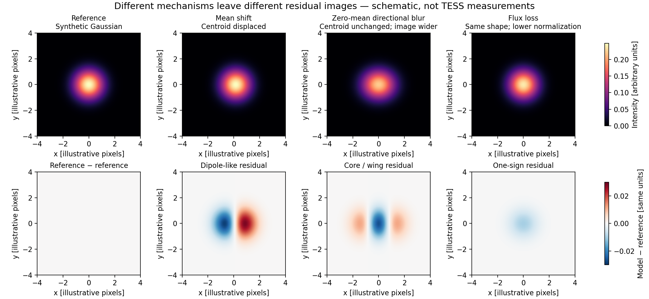
Centroid is not enough
HR 858 shows flux systematics associated with within-exposure pointing scatter and PSF width. Dispersion information can matter even when the mean location is nearly unchanged. [hr858]
A source-linked guide to spacecraft motion, changing stellar images and photometric systematics — with a practical path for TESS difference imaging.
The literature supports a layered treatment: inspect quality and engineering data, model the background, solve image geometry, allow the stellar image shape to change, then correct residual photometric correlations with signal-preservation tests. This is a synthesis of the methods below, not a single published universal recipe.
HR 858 shows flux systematics associated with within-exposure pointing scatter and PSF width. Dispersion information can matter even when the mean location is nearly unchanged. [hr858]
The handbook explains how rejecting high/low pixel samples can couple to moving starlight. The resulting flux error need not behave like a flux-conserving blur. [handbook]
A 2025 study finds high-frequency excess and time-dependent flux–position relationships in selected fast light curves. Its proposed subpixel-sensitivity explanation remains a hypothesis. [fast]
Scope: spacecraft pointing jitter and its photometric consequences. A fitted “jitter” variance in a transit likelihood and stellar radial-velocity jitter are different concepts. This is a broad, targeted review with citation chaining, not a claim to have exhaustively retrieved every TESS paper. The bibliography marks how deeply each source was inspected.
| Effect | Observable clue | What helps |
|---|---|---|
| Mean pointing drift / displacement | Field-star positions move; subtraction has dipoles | Per-exposure astrometry; registration or evaluate the model on native pixels |
| Within-exposure jitter | Quaternion dispersion, image width or ellipticity changes | Temporal PSF/ePSF or matching kernel; dispersion regressors |
| Motion × detector response / finite aperture | Flux correlates with subpixel phase or aperture choice | Better extraction; regularized centroid / pixel-based correction |
| Motion × onboard rejection | Residual flux changes with jitter despite registration | Empirical correction or rejection of poor exposures; cannot reconstruct discarded samples exactly |
| Thermal focus / background / blends | Shape change without corresponding attitude change; background structure; neighbour dependence | Independent shape, sky and scene modeling; avoid attributing all correlations to jitter |
The following is an explanatory derivation for a locally shift-invariant, linear detector, not a fitted TESS result:
Here \(t\) labels an exposure; \(\mathbf{x}\) and \(\mathbf{u}\) are detector position and displacement in pixels; \(P_0\) is a normalized static point-spread function (PSF), in pixel\(^{-2}\); \(P_t\) is its exposure-averaged form, in the same units; and \(J_t\) is the normalized displacement distribution, in pixel\(^{-2}\), estimated from pointing samples or constrained by stellar images. A PSF describes the image of a point source; an effective PSF also includes the detector response.
\(\boldsymbol\mu_t\) is the measured mean displacement in pixels; \(C_t\) is the measured displacement covariance in pixel\(^2\); \(\mathbb E_{J_t}\) denotes an exposure-weighted expectation. Mean alignment removes \(\boldsymbol\mu_t\), not \(C_t\).
Indices \(i,j\) refer to the two detector axes; \(\partial_i\) is a spatial derivative per pixel. This small-motion Taylor approximation shows why zero-mean jitter changes curvature, width and ellipticity. It neglects higher displacement moments, changing optics, saturation and nonlinear rejection. A real reference image is already blurred; matching it involves differences in blur, not convolution with the absolute jitter covariance a second time.
Flux caveat: normalized convolution conserves total flux on an infinite uniform detector. Aperture truncation, imperfect sensitivity calibration, crowding and nonlinear onboard operations break the simple inference that conserved model flux means unchanged measured photometry. A Gaussian blur is a useful baseline, not proof that all motion distributions or residuals are Gaussian.
Early attitude-control changes followed noisy wheel-speed measurements; the handbook describes improved pointing after an algorithm change. This is historical context, not a present-day jitter amplitude. [handbook] Later mission operations place momentum management differently; use the actual observation and dump tables instead of hard-coding the early cadence. [ops]
There is no single jitter-to-ppm conversion valid for every star. The coupling depends on the stellar image, detector position, brightness, neighbours, aperture and cadence. The often quoted mission noise requirement is not a measured universal residual floor. [instrument]
| Method | Supported use | Main limitation / check |
|---|---|---|
| Quality and engineering cuts [fausnaugh] | Exclude loss of pointing, anomalous excursions and unreliable epochs. Fausnaugh bins both offsets and their scatter to FFI windows. | Flag definitions and reprocessing versions matter. A clean flag does not prove clean photometry; document retained duty cycle. |
| Aperture design [condensed] | Capture moving flux and saturated bleed; compare several apertures. Mission reprocessing enlarged some bright-star apertures to reduce losses. | Larger apertures also collect more background and contaminating stars. A time-varying aperture needs its own throughput validation. |
| Centroid decorrelation [eleanor] | Fit flux dependence on image position, with low-order terms or a regularized response surface. | Does not measure motion inside an exposure. Target centroids can themselves move during genuine variability in a blend. |
| Quaternion decorrelation [hr858] | Use exposure-binned attitude statistics, especially scatter; combine with selected common trends. | Camera coordinates, missing samples and time alignment must be handled. Telemetry does not encode all local optical effects. |
| Registration + subtraction [reduce] | Effective when relative shifts dominate and cutouts do not constrain a flexible kernel well. | Residual shape changes remain; interpolation correlates pixel noise. Avoid blindly smoothing across pointing discontinuities. |
| Kernel-matched subtraction [dia] [cdips] | Match image shapes as well as positions; crowded-field surveys demonstrate practical use. | Kernel freedom competes with background, flux and transient signal. Reference choice and stellar support determine stability. |
| Empirical PSF / ePSF scene fits [tglc] [pathos] | Model neighbours and allow local image shape to change with time. | Catalogue errors, variable neighbours and an unconstrained PSF can bias flux. A better residual image alone is insufficient. |
| CBV / ensemble detrending [tda_corr] [spoc] | Fit common instrumental trends from other stars, with regularization and science-dependent settings. | Real variability can overlap the nuisance basis. Transit and asteroseismic objectives need different preservation tests. |
| Pixel regression / PLD / causal pixel model [unpopular] [pld] [pldtut] | Model shared pixel signals; distant-pixel predictors and held-out fitting can preserve slow transients. | Background dominance, contamination and predictor leakage matter. TESS Lightkurve defaults differ from K2. |
| PSF-shape components [wasp76] | Image autocorrelation/PCA can expose changes missed by centroids; demonstrated in a TESS application. | Shape is not uniquely jitter: focus and blends also change images. Select components with validation and an astrophysical model. |
| Joint GP / astrophysical fit [k2sc] [sff] [everest] | Separate position dependence from time-dependent astrophysics rather than removing all smooth variations first. | Identifiability is weak when instrument and source vary together. K2 evidence does not establish TESS performance. |
Vanderburg et al. used quaternion dispersion and fast-timescale cotrending vectors for the more affected sector, while clipping broad-image outliers in another. Their reduction masked transits when refining the correction. The result is a concrete precedent, not a universal choice of regressors. [hr858]
Inspect the original Fig. 2 and §2.1 →Kálmán et al. analyze WASP-167 in Sector 64 and report related behavior in some other fast light curves, but not all. Simple position correction reduces the high-frequency feature; different intervals show different relationships. Do not infer a fixed all-sector correction or equate this with the onboard-rejection mechanism. [fast]
Inspect original Fig. 1 →In its SN 2020fqv cutout comparison, shifts gave cleaner subtraction than the tested discrete-kernel fit. This supports checking whether the data constrain a kernel. It does not demonstrate that PSF changes are absent in every field or that all kernel methods fail. [reduce]
Inspect original Fig. 12 / Appendix A →Han & Brandt fit local ePSFs independently for each frame and use Gaia to constrain the scene. This provides a direct alternative to correcting extracted flux afterward. It does not uniquely decompose jitter, optical focus and detector response. [tglc]
Inspect model and residual figures in §III →

The 2024 WASP-76 b analysis combines engineering detrending with image-shape components. The 2026 QLP release adopts TGLC photometry from Sector 94, demonstrating continuing movement toward catalogue-assisted extraction. Neither result establishes a universal jitter-only improvement factor. [wasp76] [qlp2026]
What remains unsettled: the relative contribution of intra-pixel response, aperture leakage, onboard rejection and imperfect scene modeling for a given target; whether telemetry alone predicts its residual image; and whether a more flexible correction preserves the astrophysical signal. The studies use different targets, cadences, baselines and noise metrics, so their published precision values should not be ranked as a controlled comparison.
Recommendations inferred from this review. No SynDiff run was modified, no new TESS dataset was fitted, and no improvement is claimed for your current pipeline.
\(f_t\) is extracted relative flux (dimensionless); \(m(t;\theta)\) is the astrophysical model with fitted physical parameters \(\theta\); \(\mathbf z_t\) is a measured, centered and standardized dimensionless nuisance vector; \(\boldsymbol\beta\) is its fitted coefficient vector in relative-flux units; \(\epsilon_t\) is residual measurement noise in those units. Candidate entries of \(\mathbf z_t\) include mean shifts, within-exposure dispersion/covariance, image-shape measures, background and a small set of CBVs. These are alternatives to compare, not a recommendation to include all correlated features. Choose regularization on held-out blocks. A fitted extra white-noise term only inflates uncertainty; it does not correct the instrumental effect.
| Question | Show this evidence |
|---|---|
| Did geometry improve? | Data/model/residual stamps plus residual centroid vectors across the CCD |
| Did blur modeling improve? | Low/high-jitter absolute stacks and their differences, shared scales, matched star populations |
| Did photometry improve? | Flux residuals against mean motion and dispersion; matched-cadence scatter, PSD and time-binned residuals |
| Did it preserve science? | Pixel/scene-level injected transits and slow transients recovered through extraction and detrending; amplitude/timing bias and completeness |
| Is it robust? | Held-out magnitude, colour, position and crowding bins; quiet/poor-pointing epochs; background and focus controls |
For faint transients, prioritize scene/background fidelity and preservation of slow rises. For bright isolated stars, telemetry plus conservative extraction is a strong baseline. For crowded fields, compare catalogue-assisted PSF photometry with difference imaging. For fast cadence, also inspect the high-frequency spectrum and time-dependent coefficients. These are conditional recommendations, not measured rankings.
Start with the sector/reprocessing release notes and engineering-product inventory, then use tessvectors when its cadence and camera coverage fit the task. Its exposure-binned products are convenient but do not replace checks on sampling and timestamps. [drn] [products] [vectors]
Compare existing light curves when available: TGLC, TASOC, eleanor, and the relevant SPOC products. Agreement across independent reductions is useful; disagreement should trigger inspection of apertures, neighbours, masks and filtering.
Download the full collection as CSV, BibTeX, or JSON. PDFs link to the authors’ or archives’ copies; the report does not redistribute full papers. BibTeX entries are portable reading-list records, with publication/preprint dates retained in the notes.
Read §§8.2 and 9.2.1 for attitude-control history and jitter coupling to onboard rejection. Historical hardware description; consult release notes for later operations.
Review depth: Full PDF; relevant sections read
Source ↗Prelaunch control-system and photometric simulations. Useful physical foundation; not a measurement of present-day on-orbit residuals.
Review depth: Primary abstract / documentation inspected
Source ↗Essential reading: §2.1 and Fig. 2. Within-exposure quaternion scatter and image widths trace flux systematics; correction differs between sectors.
Review depth: Full text; §2.1 read
Source ↗Fast-cadence high-frequency excess and changing flux–centroid relationships. Jitter attribution is plausible, not a uniquely demonstrated detector mechanism.
Review depth: Full text read
Source ↗ · PDF ↗Pointing model, extraction, background treatment and systematics correction; practical centroid-regression baseline.
Review depth: Full text and author documentation inspected
Source ↗ · PDF ↗Image subtraction for transients; uses exposure-binned guiding offsets and within-bin scatter to reject poor pointing. Read reduction section and Appendix A.
Review depth: Full text; reduction section read
Source ↗ · PDF ↗Alignment, structured-background removal and calibration. Appendix A compares shifting with a discrete-kernel fit on a small cutout.
Review depth: Full text; alignment and Appendix A read
Source ↗ · PDF ↗Discrete-kernel subtraction and signal recovery on official prelaunch simulated FFIs. Do not mistake its noise-floor demonstration for an all-sector flight result.
Review depth: Primary abstract / documentation inspected
Source ↗ · PDF ↗On-orbit image subtraction and time-series processing in cluster fields; complementary to the earlier simulated DIA demonstration.
Review depth: Primary abstract / documentation inspected
Source ↗ · PDF ↗Empirical PSFs, catalogue priors and neighbour subtraction for crowded-field light curves. Addresses dilution and extraction as well as systematics.
Review depth: Primary abstract / documentation inspected
Source ↗ · PDF ↗Local ePSFs fit independently by frame with Gaia priors and background modeling; directly relevant to temporal scene modeling.
Review depth: Full text; §III read
Source ↗ · PDF ↗Reports adoption of TGLC photometry methods from Sector 94. This is a pipeline-performance update, not an isolation of the jitter contribution.
Review depth: Primary abstract / documentation inspected
Source ↗ · PDF ↗Distant-pixel predictors, ridge regularization and train/test separation; designed to preserve long astrophysical signals.
Review depth: Full text and abstract inspected
Source ↗ · PDF ↗Extraction, background, timing and bright-star halo photometry. Companion to the systematics-correction paper.
Review depth: Primary abstract / documentation inspected
Source ↗ · PDF ↗CBV and ensemble approaches for differing variability regimes; §4.5 gives use-case guidance.
Review depth: Full text and MAST product documentation inspected
Source ↗ · PDF ↗SPOC architecture and PDC context. Historical design paper; pair with current data-product documentation.
Review depth: Primary abstract / documentation inspected
Source ↗TESS extraction combines background PCA, quaternions/CBVs and PSF-autocorrelation components with an astrophysical fit. Shape diagnostics offer information beyond centroids.
Review depth: Publisher reduction-section excerpt inspected
Source ↗Independent TESS extraction with background PCA and engineering/CBV detrending; an application example rather than a global benchmark.
Review depth: Publisher reduction-section excerpt inspected
Source ↗Flux-position decorrelation foundation. K2’s motion pattern differs from TESS, so its one-dimensional motion model and performance do not transfer automatically.
Review depth: Primary abstract / documentation inspected
Source ↗ · PDF ↗Simultaneous position-dependent systematics and time-dependent stellar variability, with injection tests. Transferable method, not a TESS validation.
Review depth: Primary abstract / documentation inspected
Source ↗ · PDF ↗Regularized higher-order pixel-level decorrelation and neighbouring-star predictors. Useful for overfitting control; published performance is for K2.
Review depth: Primary abstract / documentation inspected
Source ↗ · PDF ↗Use the release applicable to the exact sector and reprocessing version, especially pointing, guiding, thermal events and excluded intervals.
Review depth: Primary abstract / documentation inspected
Source ↗Sector-by-sector operational context. Includes aperture revisions addressing jitter losses in saturated stars and historical anomalies.
Review depth: Primary abstract / documentation inspected
Source ↗Current mission planning and observation intervals; extended-mission operations differ from the early dump schedule.
Review depth: Primary abstract / documentation inspected
Source ↗Authoritative paths and filename patterns for quaternions, engineering data and other products.
Review depth: Primary abstract / documentation inspected
Source ↗Convenient camera/sector/cadence summaries, quaternion dispersion and quality. Read time-system, staggered-CCD and missing-camera caveats.
Review depth: Repository README read
Source ↗Regression, CBV and PLD interfaces; CBV regularization balances residual correlations against introduced noise.
Review depth: Primary abstract / documentation inspected
Source ↗TESS and K2 have different defaults. Check installed-version behavior and masks; an API called PLD is not automatically a dedicated TESS jitter model.
Review depth: Primary abstract / documentation inspected
Source ↗Examples and diagnosis; the TESS tutorial emphasizes background removal, while the K2 example addresses motion.
Review depth: Primary abstract / documentation inspected
Source ↗Instrument performance and cosmic-ray processing; fast-cadence products do not share the onboard rejection used for longer integrations.
Review depth: Primary abstract / documentation inspected
Source ↗Recent moving-target example using jitter regression. Specialized reduction; not evidence that a stationary-star recipe transfers unchanged.
Review depth: Primary abstract / documentation inspected
Source ↗Reviewed on 19 October 2026 using web searches across arXiv, publisher pages, institutional repositories, NASA/MAST/MIT documentation and author-maintained software. Query families covered TESS pointing jitter, quaternion moments, momentum dumps, cosmic-ray rejection, fast-cadence blue noise, centroid decorrelation, temporal PSFs, image subtraction, CBVs, PLD, causal pixel models, and 2025–2026 updates. Citation chaining connected the HR 858, TESSreduce, TGLC and later application papers.
Priority went to sources that explain a mechanism, implement a relevant treatment, or expose a failure mode. The library deliberately distinguishes direct flight evidence, prelaunch simulation, pipeline methods, operational documentation and K2 heritage. Full texts were read for key mechanisms and algorithms; other entries were screened at the primary abstract or relevant excerpt level as explicitly labeled. This is not an ADS/Scopus systematic-review export or an exhaustive citation count. Failed HTML access was supplemented with PDF/documentation where available. Search-engine “published” or crawl dates were not treated as paper dates.
No universal ppm gain or statistical confidence interval is estimated here. This report synthesizes published evidence; it does not reanalyze the underlying time series. The original schematic uses arbitrary Gaussian examples with known perturbations and is reproducible from the local generator.