PS1-assisted astrometric and chromatic ePSF calibration of TESS full-frame images
This is the working draft of Paper 1's structure and figures, in reading order. The section summaries are condensed from OUTLINE.md and the figure numbers are OUTLINE's planning identifiers. The adopted exposure is tess2020120182919-s0024-2-2 (sector 24, camera 2, CCD 2); the replication fields are S20 C3K3 and S22 C3K3. The adopted model is A3 with the moment-blind prior. All accuracy numbers must be out-of-fold. Click any figure to open it full size.
Structure (revised twice on 2026-09-30): §2 band templates mapped onto the TESS grid; §3 Preliminary de-crowded image (PS1 template matched with an empirical kernel); §4 Scene modelling (simultaneous fit of stellar fluxes, WCS and chromatic ePSF); §5 Final de-crowded image (per-band templates convolved with the calibrated chromatic ePSF), then forced photometry and targeted de-crowding. Appendices: A F=1 vs F=4, B colour model, C band-synthesis checks.
Terminology: "preliminary de-crowded image" and "final de-crowded image", not "difference image", because the bright calibration stars are deliberately still in them. The two differ only in the kernel.
Status and next steps (2026-09-30)
- Your decisions that freeze the model:
- D16 prior recipe: the bake-off is paused; fluxtruth favours moment-blind.
- D9 brightness width:
bfwidth_prodis running. - Local-background term:
localbgstep 3 is running. - C3K3 handling.
- Where the delivered ePSF comes from. Recommendation: one final fit per field on the F=4 preliminary image; D14 shows the template choice moves the WCS by 0.5 mpx, against 14 mpx split-half noise.
- A name for "targeted de-crowding".
- Final scene-model fits (F1, F2, S22; all stars plus K = 5 folds; b914ef), then regenerate §4.6–4.7 (Figs 14, 9, 11, 17, 10, 15, 12; Tables 2–3; B2).
- Per-band rebuild from the final fit (9f71e7): Figs 16, 18 (final column), 20, and S-weights.
- Targeted de-crowding (new agent): Figs 19 and 21.
- Can be made now (figure agent):
- Fig 6 background removal;
- Fig 7 "why the preliminary products are not enough";
- Fig 18 stand-in;
- App A metrics;
- Fig 3 with the D13 weights and a segment zoom;
- Table 1;
- restyled Fig 20, G6 and the learning curves.
1 Introduction: instrument calibration as a route to more science
The introduction motivates better use of the information already in individual TESS images. Position, image response and contaminating light all limit reliable measurements, and an undersampled ePSF and WCS are hard to estimate together in a crowded scene. It motivates the spatial and colour dependence of the response, introduces the complementary roles of a PS1-derived scene (removing contaminating light) and Gaia (astrometric and colour constraints), and states the single-FFI question and the quantities evaluated. It stays out of detrending, light curves and promised discoveries.
No figure planned.
2 PS1 reference scene: per-band templates on the TESS grid
This section describes the shared scene preparation once. PS1 supplies resolved scene information, but neither PS1 nor Gaia is exact TESS truth. The product is four band templates $T_b$ on the TESS grid. No ePSF appears here.
2.1 Inputs, footprint, and units
This subsection covers the TESS exposure, the PS1 bands and skycells (images, masks, uncertainties), the catalogues, the epoch and registration conventions, and the conversion from stored PS1 values to common linear flux before band combination. It keeps flux per pixel distinct from surface brightness when changing grids.
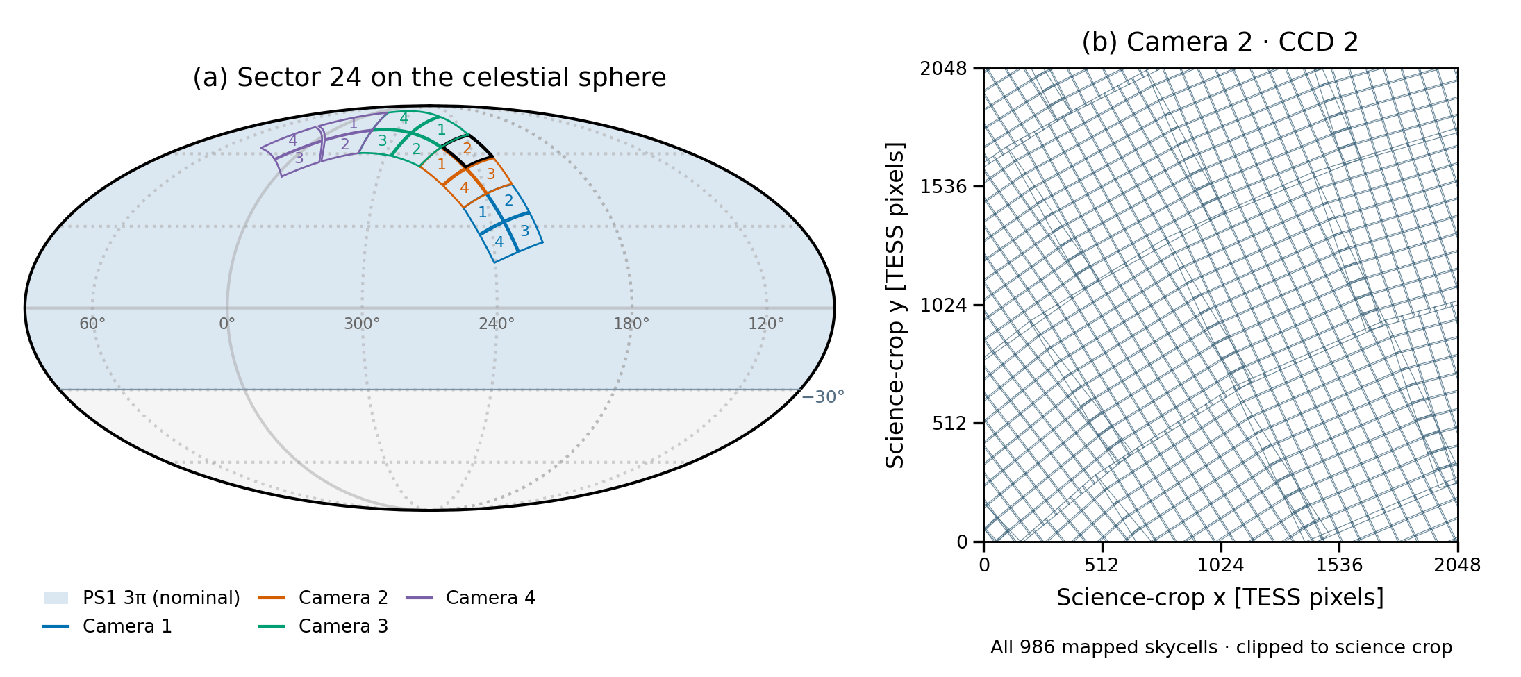
Left: healpy Mollweide view with all 16 S24 CCDs, C2K2 highlighted. Right: all 986 mapped skycell polygons in the adopted CCD's science crop. Audit: keep. The caption needs the 44-px crop offset, the WCS used (tvwcs), and the note that the F=1 mapping has 985 cells. Only the nominal PS1 extent is drawn; there is no measured usable-coverage layer.
2.2 PS1 bands and the TESS band
Main text kept short (user 2026-09-30), in four points:
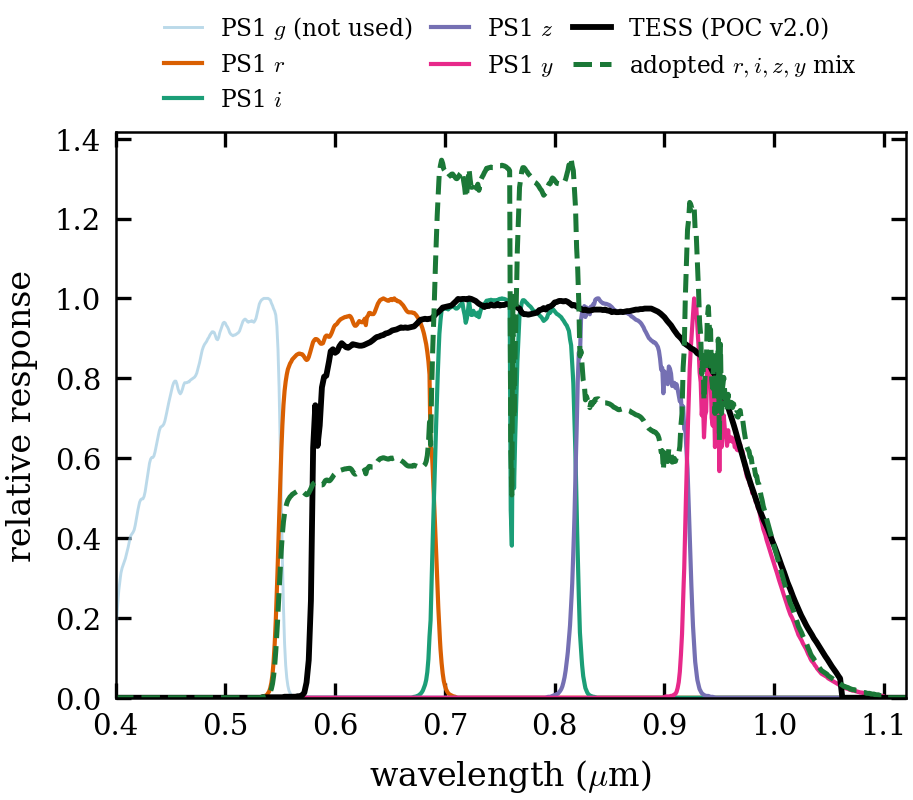
- The template is a weighted sum of PS1 $r,i,z,y$, acting as a filter that approximates TESS.
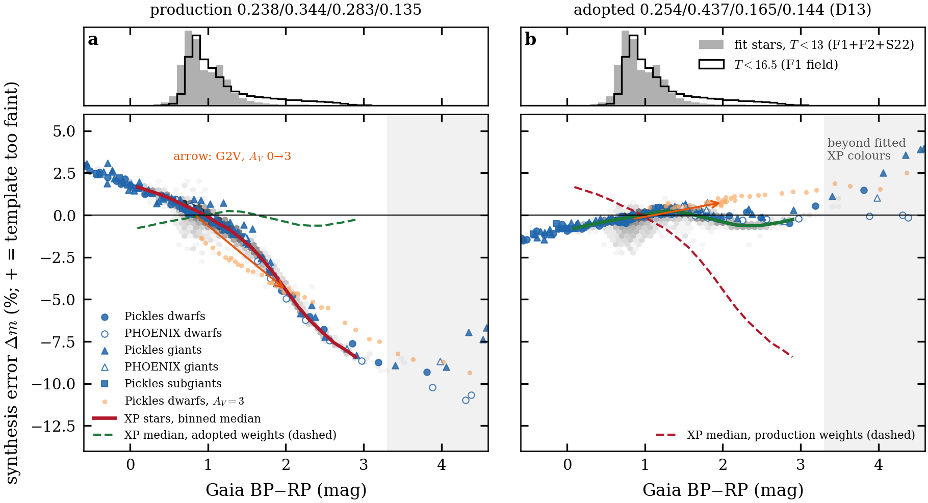
- The adopted weights are $w_{r,i,z,y}=0.254/0.437/0.165/0.144$ (D13), fitted on Gaia-XP spectra through TESS POC v2.0 (D17).
- The synthesis error is ≤0.7% held-out for stars bluer than late M; late M has a 1–2% floor.
- The match holds only when integrated over smooth spectra, so narrow emission lines are mis-weighted by ~35%.
The fit, the table by spectral type and the residual-based checks are in Appendix C. The four band templates are kept separate: their weighted sum feeds §3, and they are convolved band by band in §5.
One column: PS1 $r,i,z,y$ ($g$ light, not used), TESS POC v2.0, and the adopted mix (dashed). The mix is normalised to give the same G2V photon count as TESS and is drawn on the TESS peak scale, so its lumpy shape shows where the four-band mix over- or under-responds. The caption should state that the PS1 curves include a 1.2-airmass atmosphere (O$_2$ at 760 nm, H$_2$O at 930–970 nm) and that the mix responds at 550–580 nm, where TESS does not. The mix matches TESS only when integrated over smooth stellar spectra, not wavelength by wavelength: mix/TESS is 0.65 at 600–672 nm (including Hα), 1.33 at 717–800 nm, 0.76 at 850 nm and 0.65 at 900–910 nm. The errors cancel for stellar continua, but narrow emission lines (Hα, [S III] 907 nm) are weighted about 35% low. That goes in the §5.2 limits.
2.3 Removing PS1-saturated stars while preserving resolved neighbours
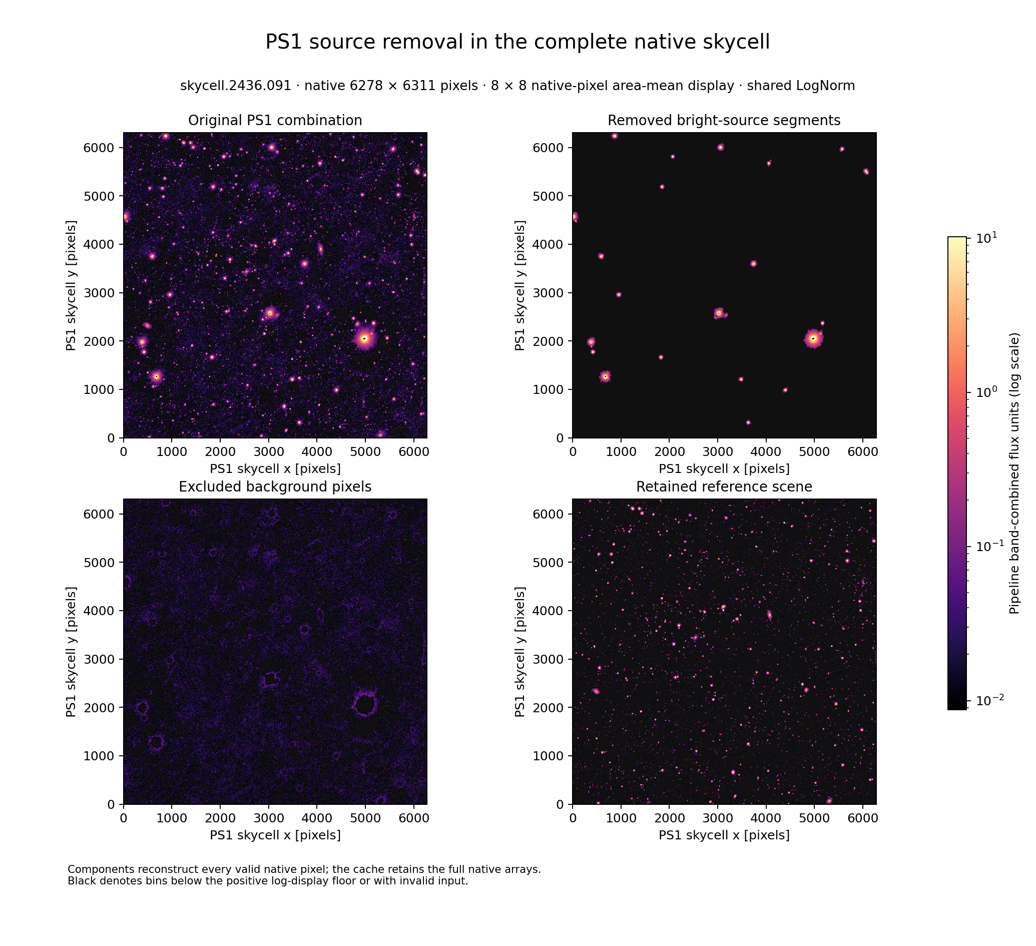
Stars are segmented in high-resolution PS1 skycell space. A bright or saturated star in its own segment is omitted, while neighbours in separate segments stay in the template even where TESS would blend them. Subtracting the template therefore exposes the omitted star in the TESS image. The same segmentation later lets any fainter target be extracted (§5.3). This subsection also states the source accounting (what is omitted, subtracted or masked) and makes the depth argument that PS1's unmodelled light is small compared with the single-FFI noise.
The full 6278×6311 skycell.2436.091 (inside the adopted CCD) is split into four components on one log scale: original, removed bright segments, excluded background, and retained scene. The components reconstruct every valid pixel. It was built with the production weights; rebuild it with the adopted D13 weights. Cosmetic fixes: drop the title and footer, name the flux unit, and explain the black saturated cores in the caption.
2.4 Smoothing and assembling a continuous scene
Gaussian preprocessing brings the PS1 response closer to the broad TESS response without depending on camera, CCD or orientation, so one prepared sky scene can be reused. This subsection keeps the PS1 PSF, the preprocessing Gaussian, the matching kernel and the final empirical ePSF distinct, and explains overlap and padding across skycells and projections (seam bookkeeping) and the flux-conserving remapping operator.
No figure planned. Relevant 09-29 finding: the production seam double-count has negligible template impact on this CCD (seam_doublecount_20260929).
2.5 Mapping the scene onto the TESS pixel grid (F=1 and F=4)
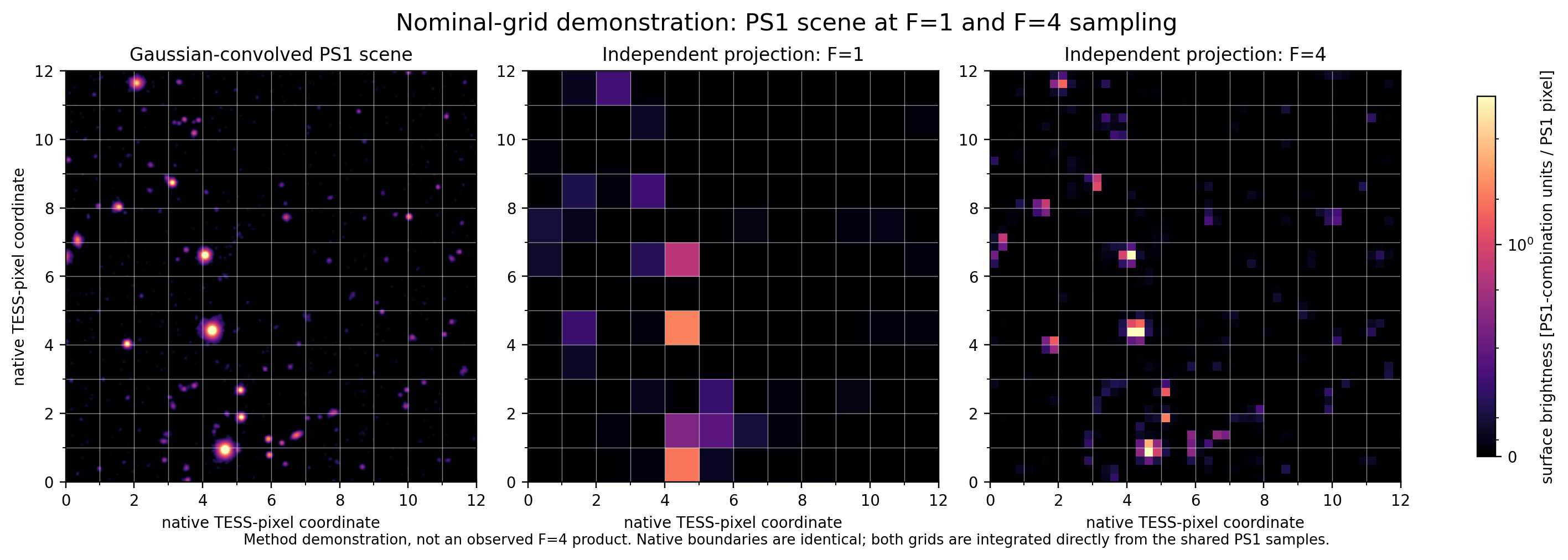
Mapping (the pipeline's mapping stage; it uses only the TESS WCS) finds the PS1 skycells overlapping the frame and assigns every TESS pixel, or sub-pixel at F=4, to one skycell, the closest centre winning in overlaps. Each band template is then the flux-conserving sum of PS1 pixels into those (sub-)pixels. Small WCS drifts become integer PS1-pixel rolls (1 PS1 px ≈ 0.012 TESS px). Because the mapping depends on the WCS, §5.1 re-runs it on the calibrated WCS. Paper 1 uses F=4. F=1 is kept for the multi-frame temporal work (Paper 2); Appendix A compares them.
A nominal-grid demonstration with a common WCS. The gridline bug is fixed (every native-pixel boundary is now drawn). It still lacks aligned source markers. The version built from real templates waits on 9f71e7's F1 rebuild with the D13 weights.
3 Preliminary de-crowded image: PS1 template matched with an empirical kernel
This section breaks the circularity. An exact template needs the TESS PSF and WCS, and measuring those needs a de-crowded image. A first match with a kernel fitted to the image itself removes enough neighbouring light to calibrate on.
Redrawn horizontally (2026-09-30): inputs and §2, then §3, §4 and §5 steps 1–4 from left to right. The dashed arrow is the optional refit, where the WCS must not shift.

3.1 The preliminary match
$$D_{\rm prel}=(I-B)-K\ast\sum_b w_bT_b$$
- $D_{\rm prel}$: the preliminary de-crowded image (native pixels, e⁻ s⁻¹).
- $I$: the FFI.
- $B$: the image-level background (§3.2).
- $T_b$: the F=4 band templates on the initial WCS.
- $w_b$: the adopted weights.
- $K$: a spatially varying kernel fitted by oversampling-aware Hotpants, which also sets the flux scale.
The template has to reproduce the PSF (spatially varying and colour dependent), the sub-pixel WCS and the flux scale, none of which is known yet. So the kernel is empirical, accepting that one kernel cannot follow a colour-dependent PSF.
3.2 Background removal: alternating kernel fits and background estimates
The sky background can't be estimated reliably on the raw crowded FFI, so it is estimated on the residual after the modelled stars are subtracted, alternating with the kernel fit, on the one adopted frame:
- A Hotpants match that includes a polynomial background term.
- A robust background estimate on $I-K_1\ast T$, with omitted bright stars and strong residuals masked and gaps filled by an exact harmonic solve.
- A second match on $I-B_1$ without a background term, then a new estimate $B_2$.
- A third, final match on $I-B_2$, which gives $K$.
- A last estimate $B$, then the final Hotpants run on $I-B$, which gives $D_{\rm prel}$.
The pipeline calls this kernel_fit; the paper doesn't use that name. Confirm the F=4 run used the same recipe.
3.3 What the preliminary image enables, and why it is not enough
What it enables: bright ($T<13$) stars omitted in PS1 space keep their TESS signal while modelled neighbours are removed. This image is the input to §4; the initial ePSF and centroids get no figure. Why it is not enough: calibration at this level leaves percent-level errors that depend on position and colour:
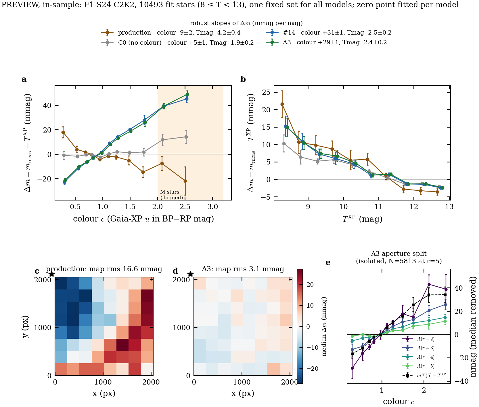
- production ePSF photometry against Gaia-XP has a ±25 mmag gradient (map rms 16.6 mmag) and a colour slope;
- the single kernel leaves a +117 mpx red−blue dipole and a red-core deficit.
If such errors vary in time, they become light-curve trends that must be detrended. This paper does not make light curves (Paper 2). It removes the static position- and colour-dependent part in one exposure, which is the prerequisite.
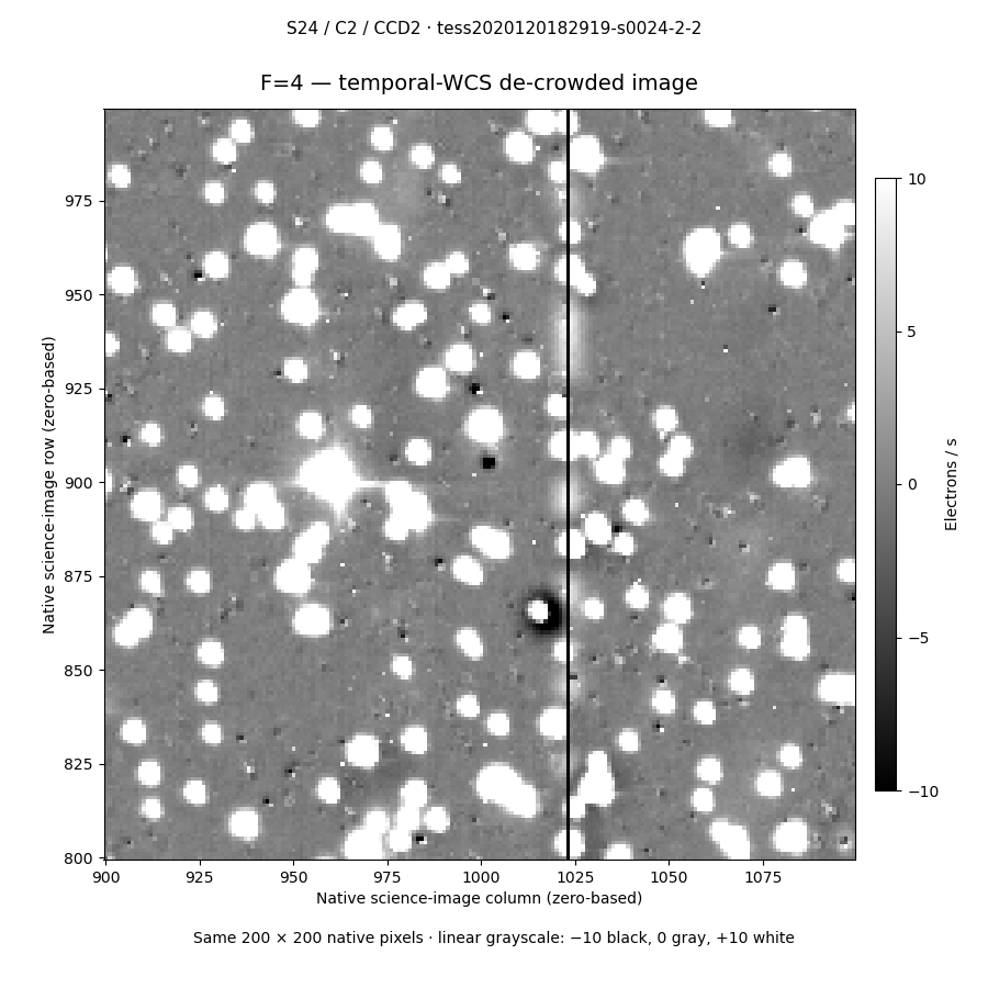
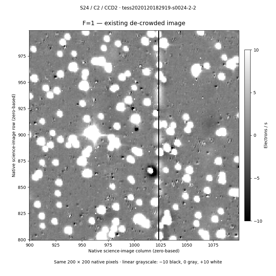
Adopted frame, F=4 Hotpants image. The bright stars stay as saturated white blobs, as intended, while fainter neighbours are removed down to small residuals. A bad column at x ≈ 1023 and a dark ring around one star near (1015, 865) are visible. The real Fig 18 adds FFI, model and final columns for 3–4 chosen stars.
4 Scene modelling: simultaneous fit of stellar fluxes, WCS and chromatic ePSF
This section fits the preliminary de-crowded image with a forward scene model: every star is rendered at its Gaia position with a spatial, colour-dependent ePSF, and its flux is fitted. There is no local background, and a matched colour-independent fit is the baseline. The model ladder is in Appendix B.
4.1 The scene model and stellar fluxes
Each star's flux is a parameter, solved conditionally (linear least squares at fixed WCS and ePSF). Bright ePSF contributors ($8\le T<11$) and fainter WCS anchors ($T<13$) constrain different parameters, and neighbours get fluxes only. The fitted fluxes are the delivered bright-star photometry; their accuracy is quoted held-out (§4.6).
Given a star's sky position, colour, flux and detector location, the model predicts native pixel values:
$$m_p=\sum_i f_i\,E\!\left(\boldsymbol p-\boldsymbol q_i;\boldsymbol r_i,\delta_i,\boldsymbol\theta\right),\qquad \boldsymbol q_i=W\!\left(\boldsymbol s_i(t_{\rm exp});\boldsymbol a\right)+\Delta\boldsymbol x_i(\delta_i,\boldsymbol r_i)$$
- $m_p$: model value of native pixel $p$ (e⁻ s⁻¹).
- $f_i$: flux of star $i$, solved conditionally at fixed shared parameters.
- $E$: native-pixel response rendered from the stored 4×-oversampled profile $P$.
- $\boldsymbol s_i(t_{\rm exp})$: Gaia position propagated to the exposure epoch.
- $W$: reference-colour WCS (tangent plane plus a degree-5 Chebyshev correction, coefficients $\boldsymbol a$).
- $\boldsymbol r_i$: detector position.
- $\delta_i$: colour offset from $c_{\rm ref}$ (Gaia-XP $u$ in BP−RP units).
- $\Delta\boldsymbol x_i$: A3 colour displacement toward or away from the optical axis.
- $\boldsymbol\theta$: the 6×6 node ePSF and the colour-shape terms.
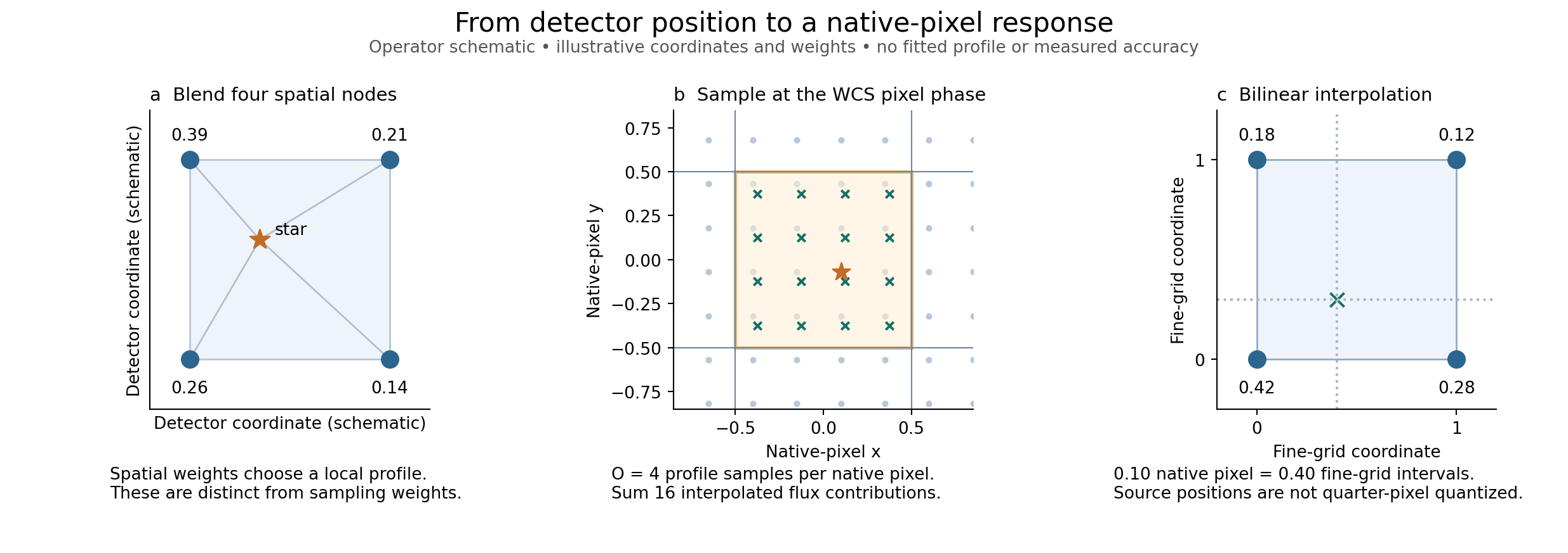
Rendering blends the four surrounding node images, evaluates 16 sub-pixel samples per native pixel at the exact WCS phase with bilinear interpolation, and sums them. Positions are not quantised to quarter pixels.
4.2 Astrometry: Gaia positions and the WCS
Gaia DR3 positions are propagated to the exposure epoch and projected with a reference-colour WCS: a tangent plane plus a degree-5 Chebyshev distortion. A star of another colour sits at the WCS position plus the chromatic displacement of §4.4, so a FITS header alone cannot encode source positions. The ePSF's core-centroid origin fixes the position gauge, so an ePSF translation cannot trade against the WCS. There is one static WCS per exposure; its time dependence is Paper 2. Held-out accuracy is in §4.6.
4.3 The spatial ePSF and rendering onto native pixels
A 6×6 grid of 4×-oversampled node images is blended bilinearly across the detector, with the moment-blind fine-neighbour prior. Rendering evaluates 16 sub-pixel samples per native pixel at the exact WCS phase and sums them.
Three operator schematics with illustrative weights: (a) blend four spatial nodes; (b) 16 sub-pixel samples at the WCS phase; (c) bilinear interpolation. It shows no measured profile.
4.4 Colour: the Gaia-XP colour and the chromatic ePSF
Each star's colour is Gaia-XP $u=\sum_b s_b\lambda_b$ (band-share-weighted effective wavelength, in BP−RP units per CCD; BP−RP fallback for about 1% of stars). Its offset is $\delta=c-c_{\rm ref}$. The A3 chromatic model has 17 coefficients per CCD, in two parts:
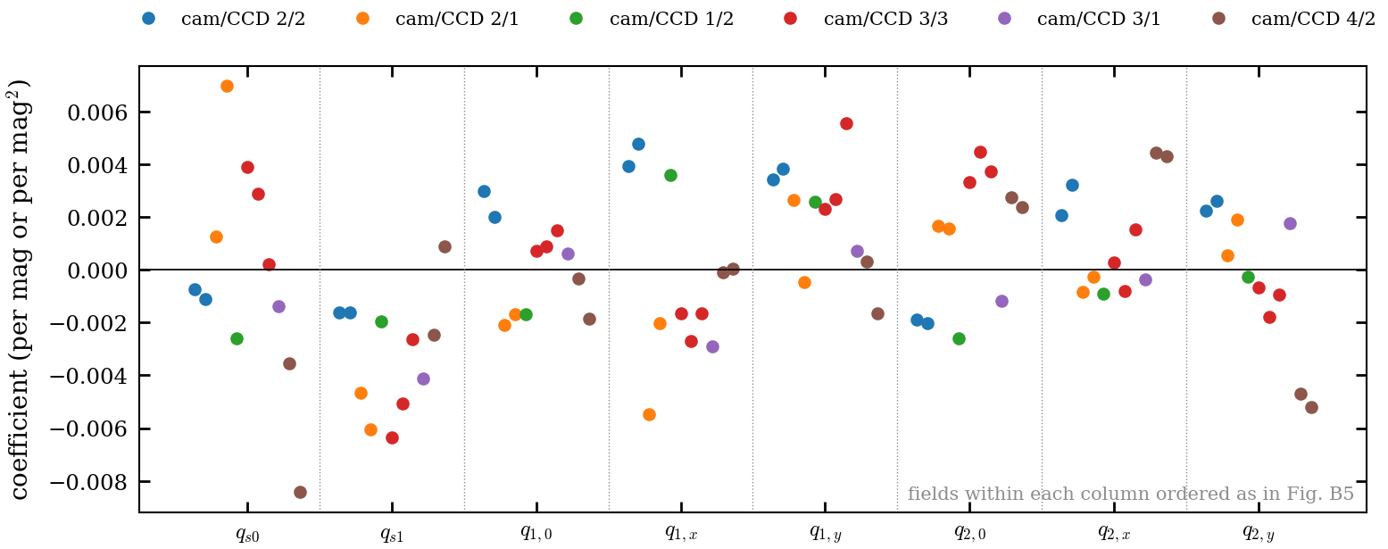
- A radial colour shift toward or away from the tess-point optical axis, quadratic in colour and in distance: $\Delta\boldsymbol x=[\delta(s_0+s_1r+s_2r^2)+(\delta^2-\langle\delta^2\rangle)(q_{s0}+q_{s1}r)]\hat{\boldsymbol n}$.
- Colour shape terms: radial kurtosis, dilation, blur and trefoil, plus CCD-frame elongation planes, all projected off $P_0$ so flux cannot trade with colour.
Symbols: $r$ is the axis distance in kpx and $\hat{\boldsymbol n}$ the unit vector toward the axis. The linearisation $E(c)\approx P_0+\delta P_1$ is what §5.2 uses. Full equations: Appendix B.
4.5 Fitting and evaluation
This subsection covers the calibration sample and parameter roles (bright ePSF contributors, faint WCS anchors), the pixel objective, noise and regularisation (moment-blind fine-neighbour prior), the conditional flux solve, and the fitting sequence. The evaluation rules are stated before any results. The delivered calibration is always trained on all stars, and overfitting checks always use K = 5 spatial folds (D19). Every quoted metric is out-of-fold (G1), with leak-free initialisation and fixed evaluation star sets shared by all compared models. In-sample numbers appear only as the memorisation ratio.
Median core χ² relative to the leak-free initial ePSF during training, by T bin. In-sample stars (red, dashed) improve steadily, while held-out stars (solid) get worse, most for bright stars and for K = 2. The single-FFI ePSF memorises its trainees, which is why the product is trained on all stars and checked with K = 5 (D19). Restyle once the recipe is final.

heldout_harness_20260929/folds/.4.6 Results: spatial ePSF, WCS and bright-star photometry
This subsection shows what spatial calibration the de-crowded image supports and how accurately it predicts positions and pixels. It covers the reference-colour ePSF across the CCD, WCS corrections kept distinct from held-out accuracy against Gaia, and the colour-independent baseline for §4.4. The brightness-dependent width is gated on G2: it goes in the model if it lowers the held-out flux error against Gaia-XP on both fields, and otherwise it is reported as a limit.
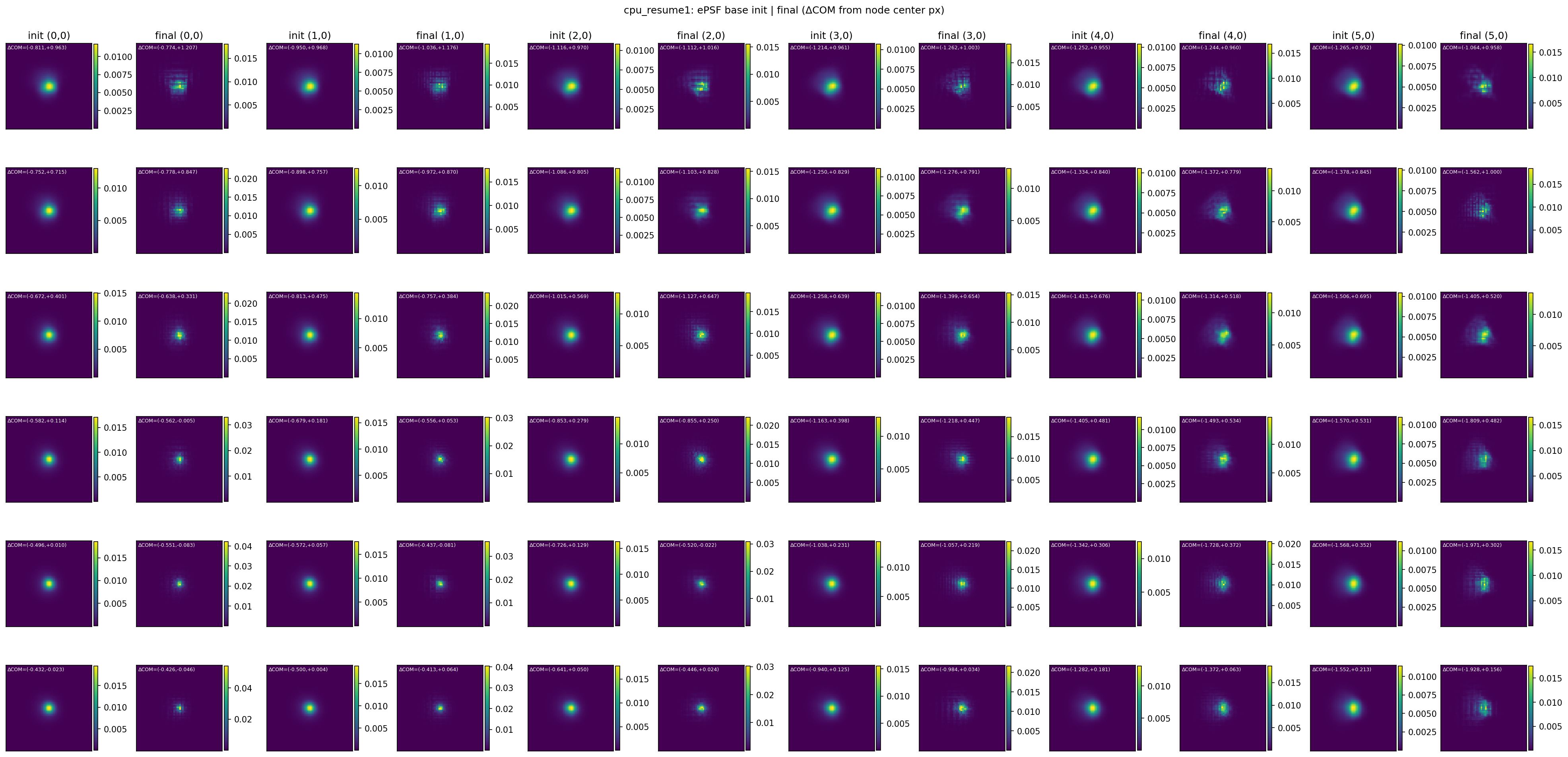
The current candidate is the 6×6 node mosaic from the 09-23 minbg fit on the adopted frame (before A3). The spec asks for a 5×5 display at fixed positions with a common phase, normalisation and stretch, plus cuts at three positions. Regenerate from the A3 + moment-blind calibration once D16 settles.
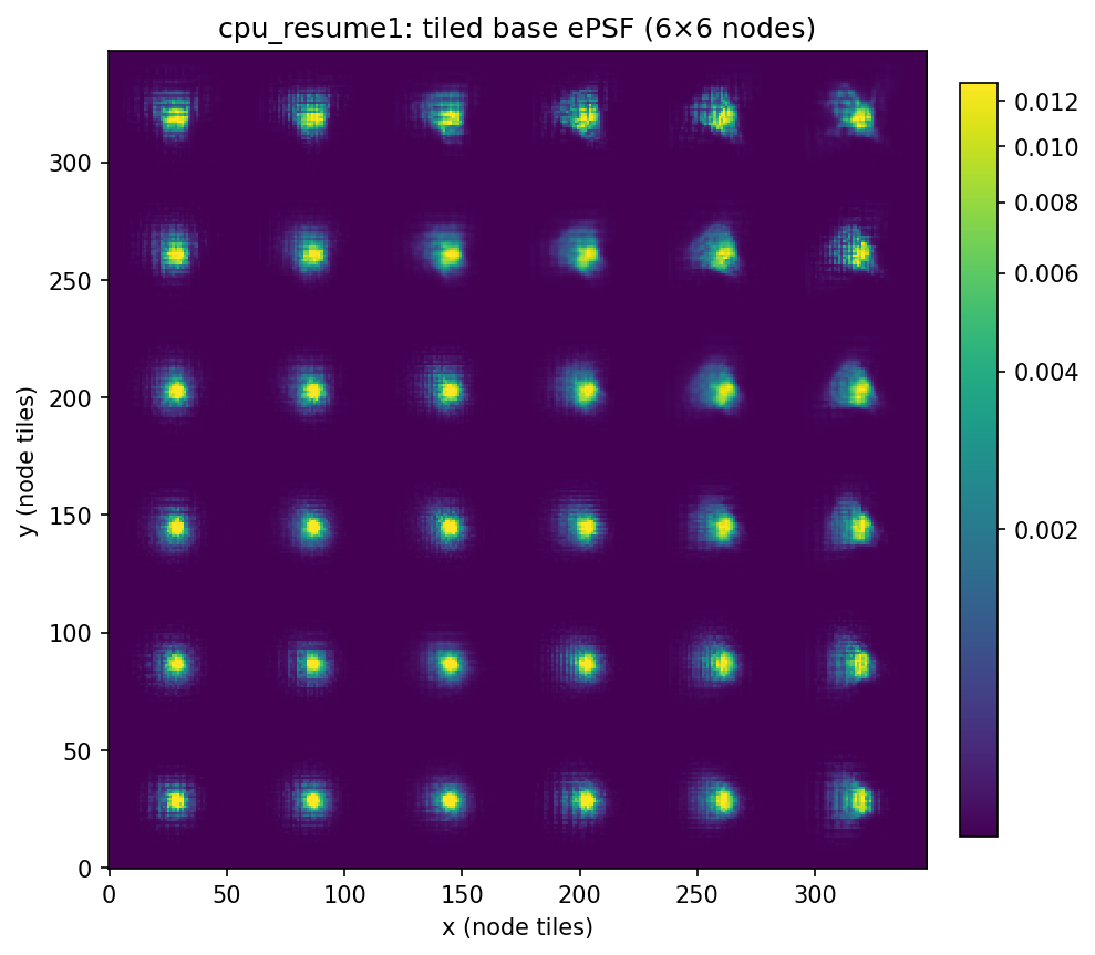
Supporting: initial vs fitted node ePSFs (6×6, in-sample)
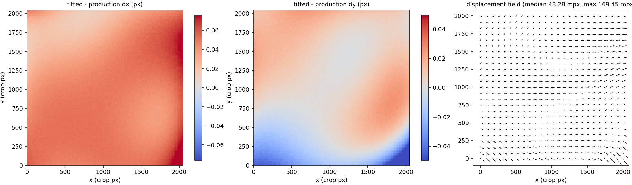
What exists compares the fitted WCS with the production WCS on the adopted frame: median 48 mpx, maximum 169 mpx, largest in the bottom-right corner. That is a comparison between solutions, not held-out accuracy. The real Fig 9 uses held-out residual-vector maps for the colour-independent and adopted fits, plus the cumulative radial error, from the G1 held-out tables.
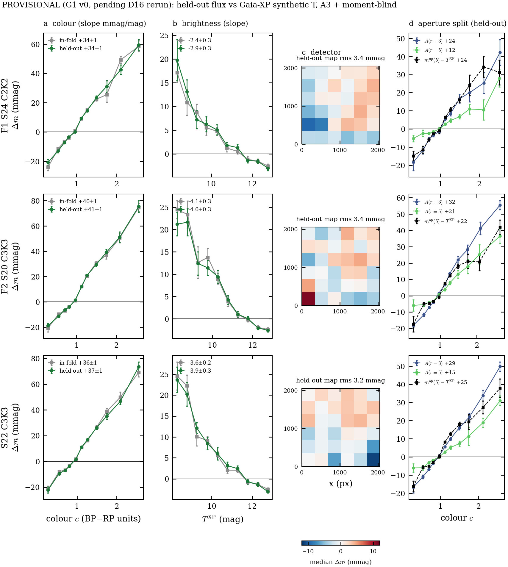
model_complete/figure11_native_model_comparison.png). Inputs: full_xsec plus folds.$\Delta m = -2.5\log_{10}F + Z - T^{\rm XP}$, where $F$ is the held-out flux (e⁻ s⁻¹), $Z$ is one fitted zero point per field, and $T^{\rm XP}$ is the Gaia-XP synthetic TESS magnitude through the POC v2.0 response. The aperture correction is $A(r)=m^{\rm psf}-m^{\rm ap}(r)$, with apertures of radius $r$ px measured on the fitted stamps. Held-out colour slopes: F1 +34, F2 +41, S22 +37 mmag/mag, the same as in-fold. The aperture-vs-XP term (+22 to +25 at r = 5 px) and the model's own aperture correction (+12 to +21) each carry part of it, so G5 is partly data-vs-XP and partly model wing normalisation. All models share a brightness term of −3 to −4 mmag/mag. The Δm map rms is 3.2–3.4 mmag. Placement (2026-09-30): this is §4.3's bright-star photometry. The delivered fluxes come from the joint fit; accuracy is quoted from held-out stars, whose flux is re-solved with the calibration fixed from the other folds, which is forced photometry. This is the T < 13 fit-star sample. The faint 13 ≤ T < 16 sample comes from extracted stars in §5.4. It is also evidence for §4.4 (colour) and §6.2 (limits). Pending the D16 rerun.
In-sample preview on F1 with production, C0, #14 and A3
4.7 Results: chromatic response
This subsection starts from the colour-dependent residuals of the colour-independent fit: blue-minus-red registered stacks with matched populations. It then explains the adopted A3 model: #14's nine global terms in distance to the optical axis, plus a quadratic-in-colour radial shift and CCD-frame colour elongation planes, with Gaia-XP colour $u$ (17 colour parameters per CCD). It measures displacement in independent colour bins, compares held-out positions and pixels between models, and tests the alternatives to an instrumental interpretation (bandpass mismatch, neighbours, background, interpolation). Known limits: the camera-2/CCD-2 width band on F1, and the red-end shift beyond 1800 px.
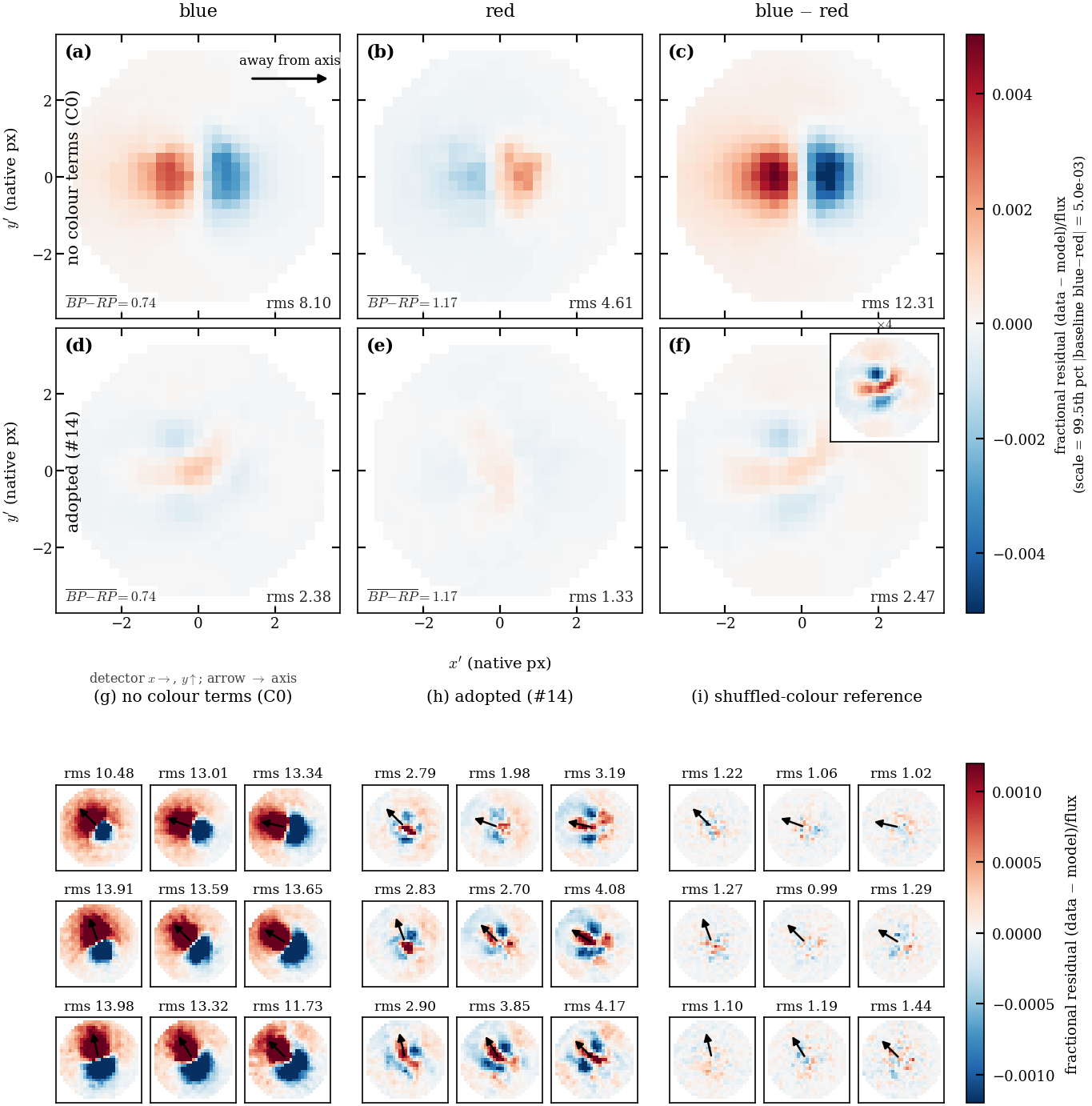
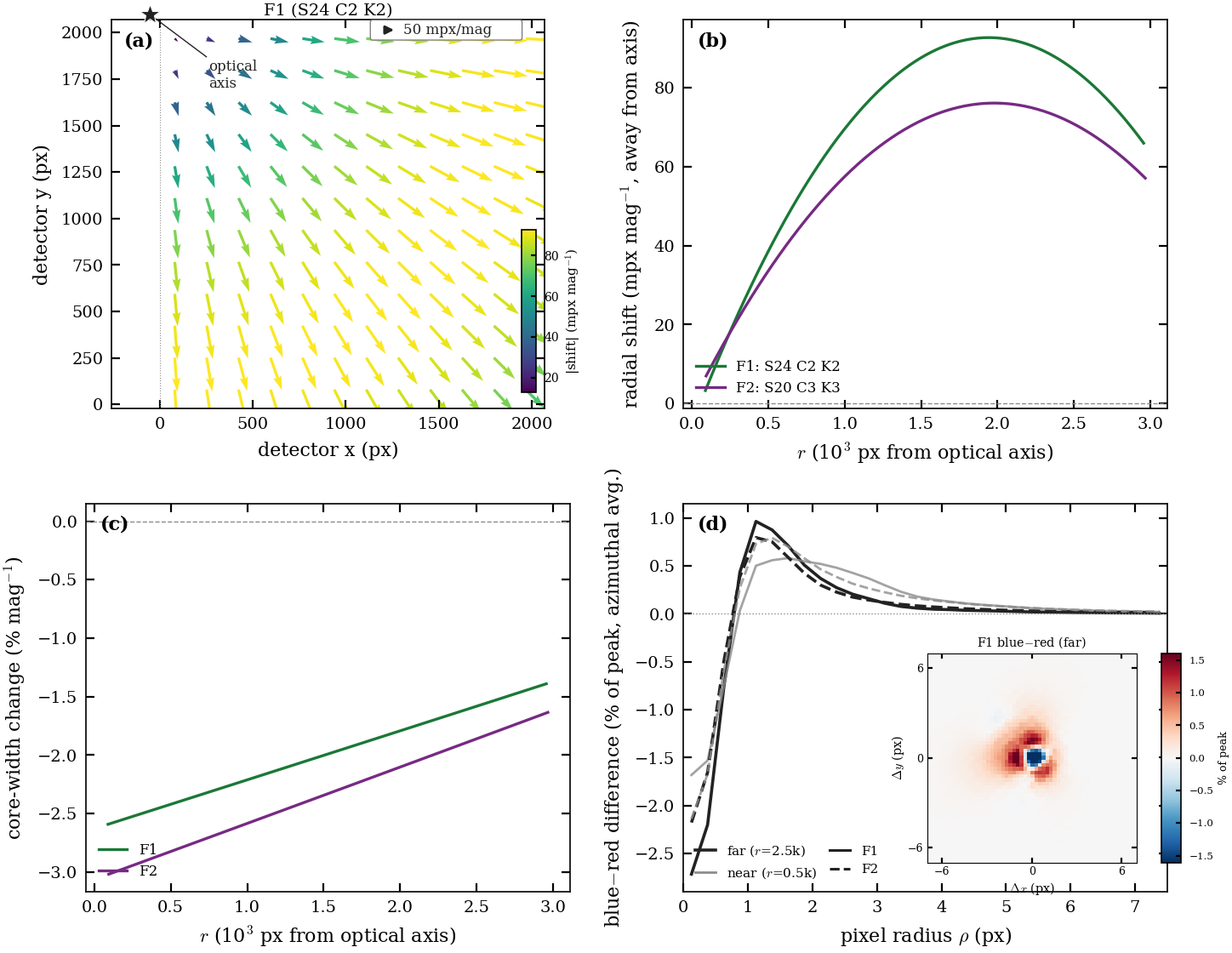
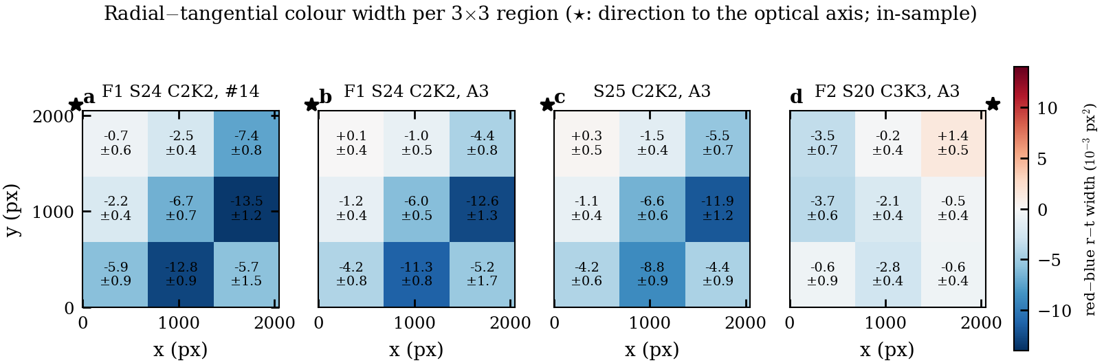
Model #14 on F1, in-sample. The blue−red residual stack drops from rms 12.3 (no colour terms) to 2.5 (#14), against a shuffled-colour floor of about 1.0–1.4. The per-cell stacks (bottom) show the dipole pointing along the axis direction in every cell. Regenerate for A3, held-out.
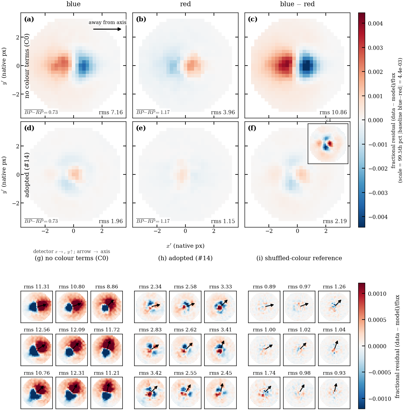
F2 replication (S20 C3K3)
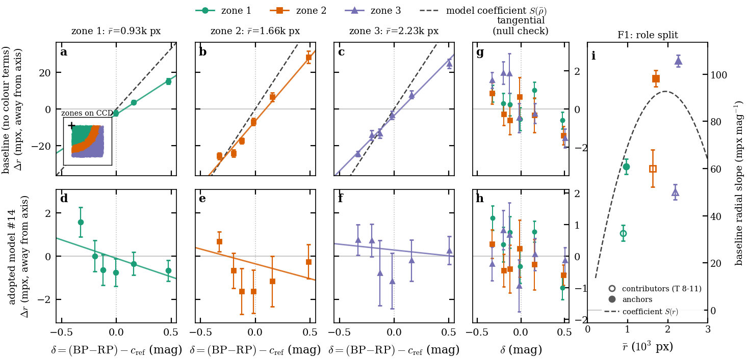
Radial displacement against colour in three distance zones. The no-colour fit shows +15 to +28 mpx at δ = +0.5; #14 flattens it to within ±2 mpx. The tangential null checks are flat. Panel (i) shows the role split (contributors vs anchors), which is limit D11. Regenerate for A3: the quadratic term is meant to bend the red end.
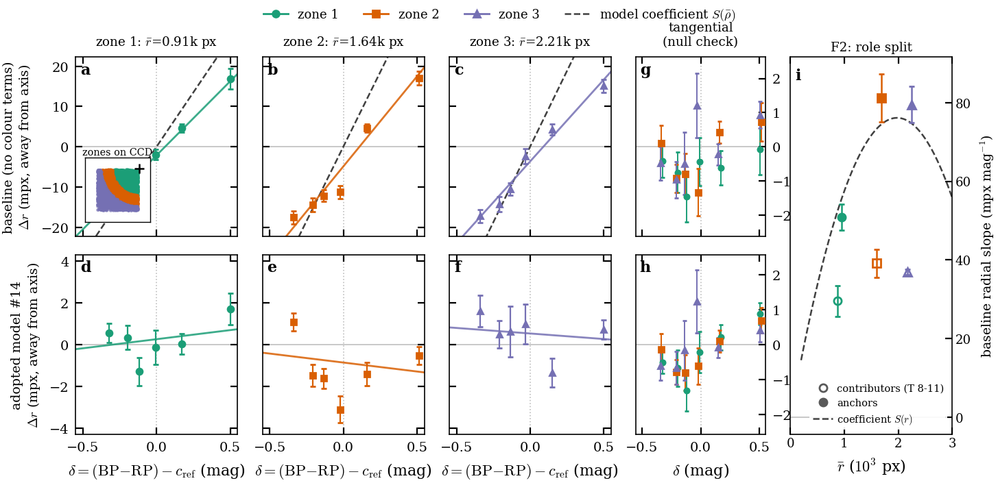
F2 replication
#14 fields: (a) shift vectors pointing away from the optical axis; (b) radial shift peaking near 90 mpx/mag at about 2 kpx; (c) core width −1.5 to −3 %/mag; (d) blue−red profile difference. The A3 version adds the per-CCD elongation planes (Appendix B6) and the quadratic shift.
5 Final de-crowded image: per-band templates convolved with the calibrated chromatic ePSF gated · G4
This section uses the trained WCS and ePSF. The template is first remapped on the calibrated WCS; then each band is convolved with its own chromatic kernel; then stars are measured by forced photometry. Nothing new is fitted except an optional verification refit.
5.1 Remapping the band templates on the calibrated WCS
The mapping of §2.5 is re-run with the §4 WCS and the F=4 band templates are rebuilt. The template WCS must equal the ePSF WCS: Phase A found a 0.047 px offset otherwise, and in Phase 1 the template and A3 WCS differed by 3 mpx median and 16 mpx maximum.
5.2 Per-band kernels from the chromatic ePSF
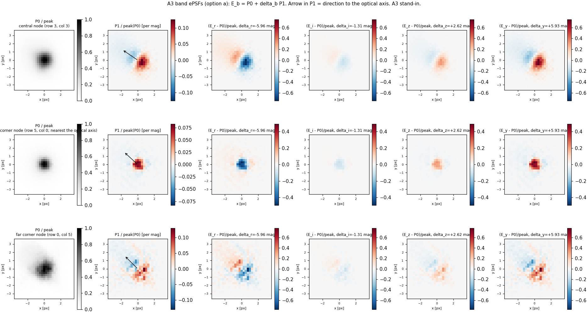
$$E_b=E(\,\cdot\,;\boldsymbol r,c_b)\approx P_0+\delta_b\,P_1$$
Here $c_b$ is band $b$'s effective colour in BP−RP units, $\delta_b=c_b-c_{\rm ref}$ is recalibrated for the adopted weights (D18), $P_0$ is the reference-colour ePSF and $P_1$ its colour derivative per mag.
$P_0$, $P_1$ and $E_b-P_0$ at three nodes: centre, the corner nearest the optical axis, and the far corner. The arrow points to the axis. $P_1$ is a dipole along the axis direction. The $r$ and $y$ kernels differ from $P_0$ by opposite dipoles of up to about 0.6 of the peak, and $i$ is nearly $P_0$. One Hotpants kernel cannot represent this spread. Restyle from the final kernels.
5.3 The final de-crowded image
$$D_{\rm final}=(I-B)-\sum_b w_b\,(E_b\ast T_b)$$
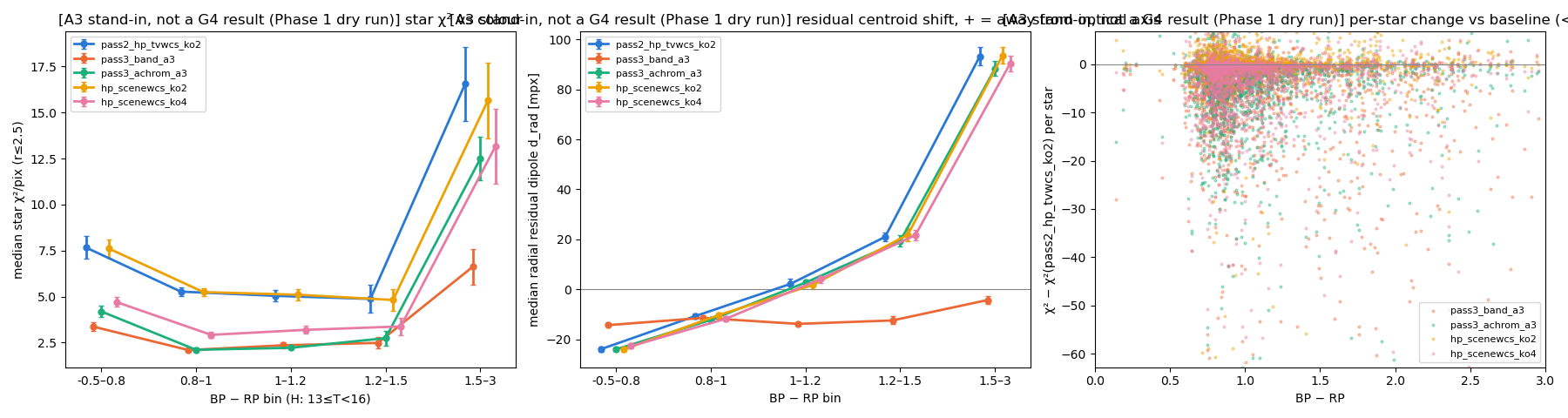
Only the kernel changes relative to $D_{\rm prel}$, so every PS1 source is rendered with the PSF for its own colour. The two images are compared on held-out stars and an unseen frame.
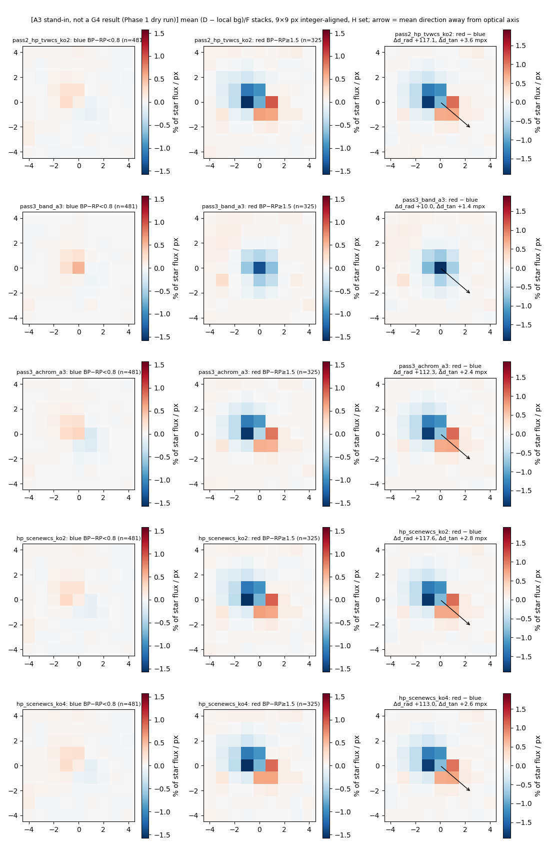
This is 9f71e7's Phase 1 whole-CCD dry run with A3 as a stand-in, not a G4 result. Red-minus-blue residual stacks: the red−blue dipole falls from +117 mpx (Hotpants, the preliminary match) to +10 mpx (per-band A3). The achromatic A3 control keeps the dipole (+112). The per-band image lowers the per-star χ² in every colour bin; the red-core deficit that remains is mostly the D13 band-weight effect, with −1 to −3% from A3 over-sharpening red stars. The final figure uses the frozen fit, the F1 rebuild, and held-out stars.
Colour-split residual stacks (5 variants)
5.4 Optional: re-running the scene model on the final image (verification)
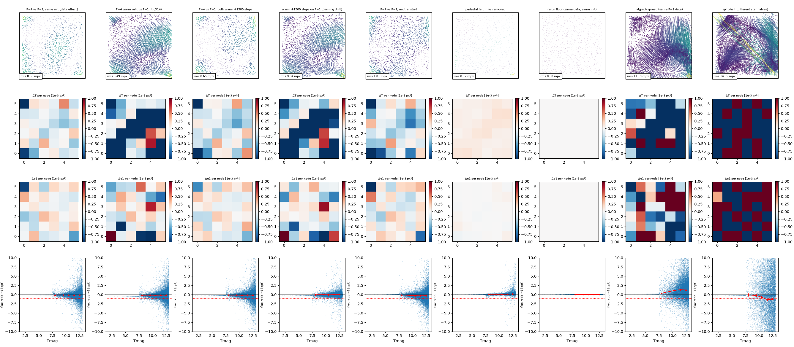
The §4 scene model can be re-run on $D_{\rm final}$ to refine the ePSF and WCS. Its main value is verification: the WCS must not shift (D14/G6).
Columns compare pairs of fits on F1. Rows show the position-difference field (rms), per-node width and ellipticity changes, and flux ratio against Tmag. Switching the input from F=1 to F=4 at the same start moves positions by 0.53 mpx rms (0.65 after both train 1500 more steps; 1.0 from a neutral start). That is well below the training drift (3.0–3.5 mpx), the init/path spread (11 mpx) and split-half noise (14 mpx). Flux ratios stay within ±0.3 ppt. So the template does not move the calibration. Restyle as one compact figure or a table for the paper.
5.5 Forced photometry and targeted de-crowding (name to confirm)
Forced photometry measures fluxes on the final image with the calibrated ePSF and WCS held fixed, at each star's Gaia position and colour. It applies directly to the bright stars, which are never in the template. Fainter stars are in the template and need targeted de-crowding first (the pipeline's "star" branch; working name):
$$M_t=\sum_b w_b\,(E_b\ast S_b^{(t)}),\qquad D_t=D_{\rm final}+M_t$$
- $S_b^{(t)}$: the PS1 band-$b$ image masked to target $t$'s segment.
- $M_t$: the target's modelled TESS image at the PS1 epoch.
- $D_t$: the targeted de-crowded image, with the target's light restored and its neighbours still removed.
This works because convolution is linear, and it is exact only with the same kernels that built the template.
5.6 Limits
- Camera 3 / CCD 3: red stars are fainter than the v2.0 prediction in every product (Appendix C, S-weights); handling is your decision.
- The per-band red-sharpening core is larger on C3K3 (−3.9…−5.6% vs −2.2…−3.4%).
- PS1 segmentation failures.
- Neighbour variability between the PS1 and TESS epochs.
6 Discussion and conclusions
This section explains what the calibration enables, bounds its interpretation, and closes the paper without a separate results recap. No new main figure is planned; it refers back to Figs 8, 14, 9, 10–12, 15 and 17.
6.1 What PS1-assisted single-image calibration enables
This subsection draws together the contributions of resolved-scene preparation, de-crowding, Gaia-constrained geometry and the colour-dependent response, each tied to its §3–4 evidence. Keeping observed bright-star profiles while suppressing modelled neighbours is what makes calibration possible in crowded images. The deliverables are a reference-colour WCS, a spatial ePSF, a colour correction, the valid region and colour range, and a reproducible configuration. It does not claim light-curve gains.
6.2 Interpretation and limits
This subsection separates evidence from optical hypotheses and bounds applicability by detector, magnitude, colour, crowding and PS1 coverage. Limits to state:
- F1's mid-distance radial−tangential colour-width band on camera 2 / CCD 2 (D5, Fig B7).
- Role- and brightness-dependent colour displacement (D11, to be rechecked on A3).
- The per-star residual floor.
- The brightness width, if G2 fails.
- The Gaia flux colour slope (G5; Fig 17 splits it into a data-vs-XP part and a model aperture-correction part).
- The residual template synthesis error with the adopted D13 weights (≤0.7% held-out; late M is the four-filter floor; about +1% for $A_V\approx3$).
- Narrow emission lines in host galaxies (Hα, [S III] 907 nm) are weighted about 35% low by the four-band mix, because it matches TESS only for smooth spectra.
6.3 Temporal extension and concluding findings
This subsection briefly motivates Paper 2: the time-varying sky-to-detector mapping (velocity aberration, pointing jitter, thermal focus) kept distinct from physical distortion. It ends with a short list of verified findings. If G4 fails, the per-band template (§5) becomes an outlook paragraph here. There is no temporal figure.
Appendix A · F=1 vs F=4 sampling
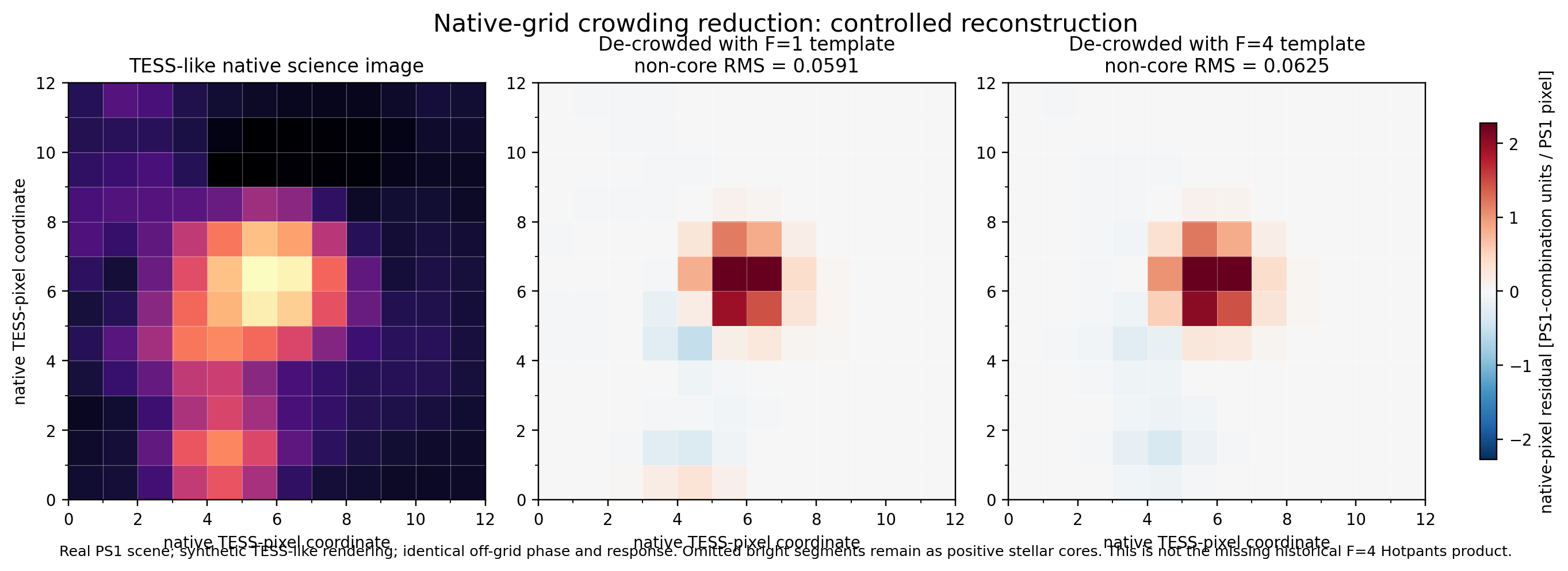
This compares the F=1 and F=4 preliminary de-crowded images on the same frame and settings, with held-out metrics. It explains why Paper 1 uses F=4 and why F=1 is kept for Paper 2.
Same frame, same display scale. The F=1 image shows many more small black-white residual pairs around faint neighbours, the signature of sub-pixel template misregistration, than the F=4 image. The bright-star cores and the bad column look the same in both. Held-out metrics are still to be computed.
This is a controlled reconstruction: a real PS1 scene rendered as a synthetic TESS-like image, not an observed F=1/F=4 product. The non-core RMS is similar (0.059 vs 0.063). The real version needs the F1 F=4 product from 9f71e7 and aligned native-grid outputs for the same stars.
Appendix B · Selecting the chromatic ePSF model
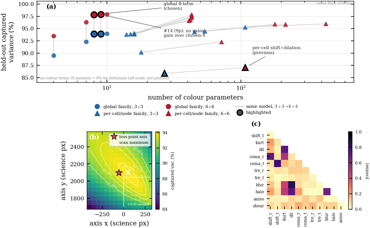
This appendix records why these colour terms were chosen, why they are global rather than per-node, and which fitting choices the result depends on. B.1–B.5 cover the #14 selection. The new B.6 covers the step from #14 to A3. All of this is in-sample model-selection evidence on fixed star sets.
B.1–B.3 Candidate terms, selection diagnostic, held-out colour-half selection (#14)
There are 12 candidate generators, several of them collinear. The selection score is the blue−red stack against a shuffled-colour reference, not the loss. A global 8/9-term model in distance to the axis captures about 94% (3×3 cells) and 98% (6×6) of the held-out colour variance, better than per-cell freedom. The data fix the direction to the optical axis, not its distance.
B.4 Trained ablation on two fields (#14)
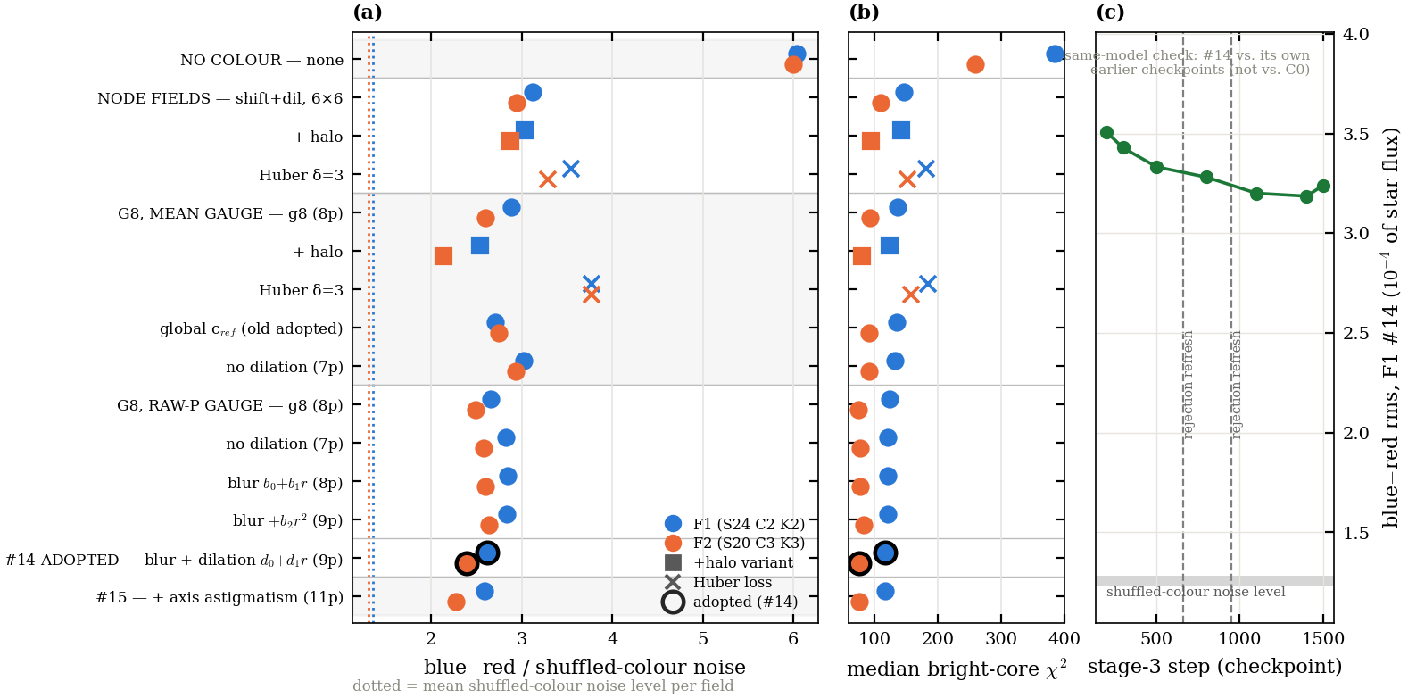
Sixteen variants were retrained on F1 and F2. The blue−red leftover goes from 6.0 (no colour terms) to 2.6/2.4 (#14). #15 (adding axis astigmatism) gains less than the run-to-run scatter. The median bright-core χ² tracks the same ordering, and the model is converged to about 0.05.
B.5 Fitting choices the colour result depends on
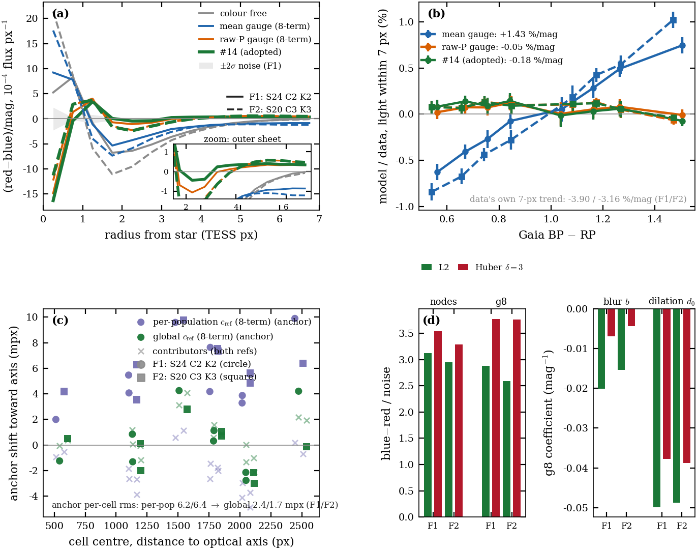
Three choices matter. The raw-P gauge removes the flat colour sheet that the mean gauge leaves (a +1.4 %/mag aperture bias). One global $c_{\rm ref}$ avoids a role-dependent shift. L2 beats Huber, which down-weights bright cores.
B.6 From #14 to A3 (new)
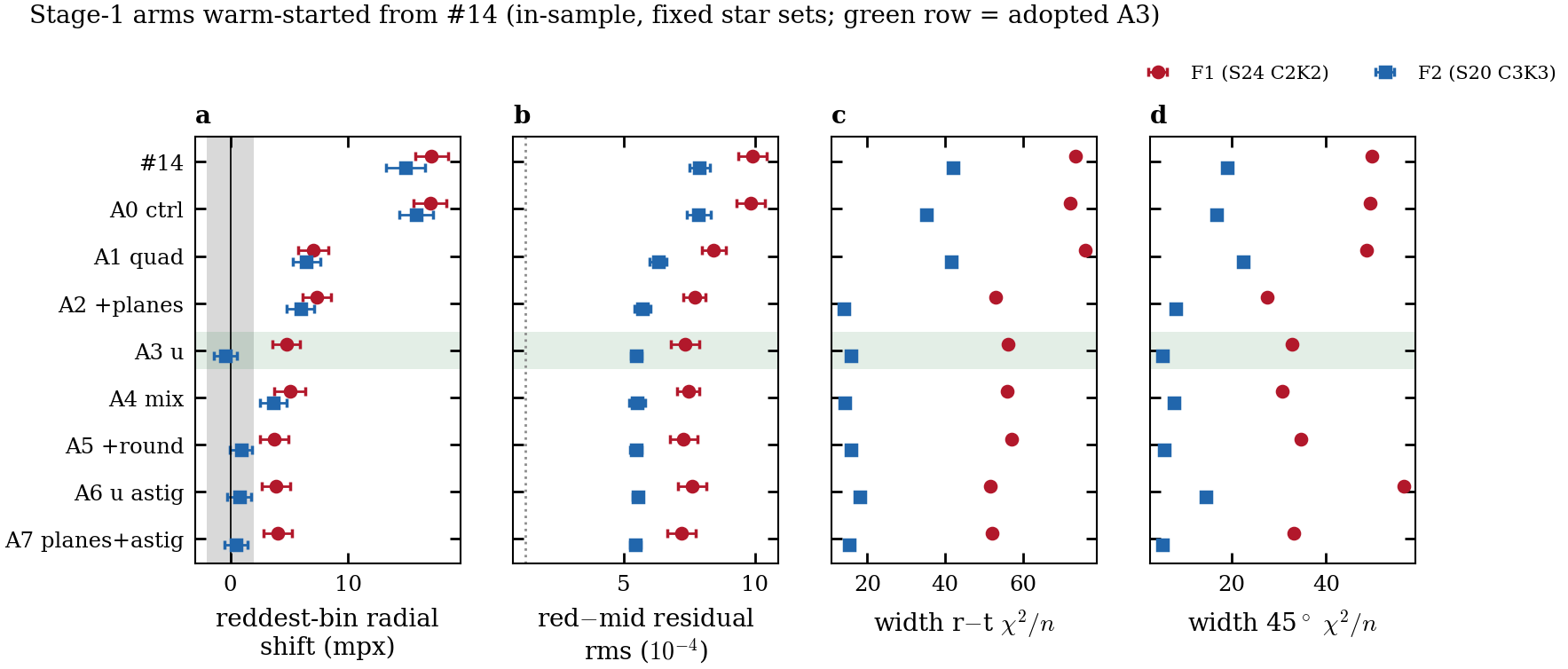
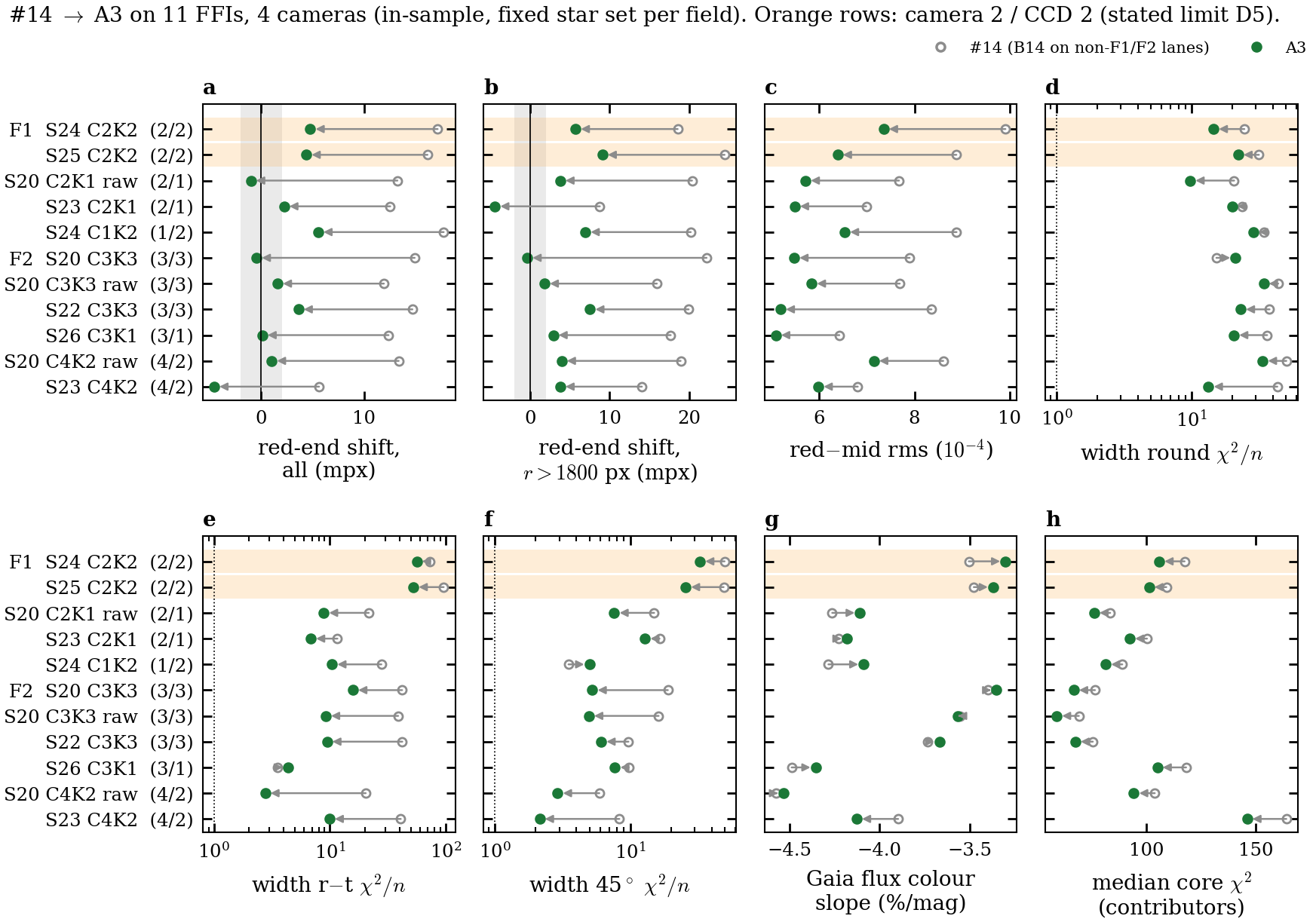
Stage-1 arms on F1 and F2, then #14→A3 on 11 FFIs across four cameras. The quadratic shift halves the red-end shift, $u$ takes F2's red end to −0.4 mpx, and the planes fix the width everywhere except camera 2 / CCD 2. Draft text and captions: figures/chromatic/a3/APPENDIX_B_A3_NOTES.md. Table B2 (17 coefficients) should be refreshed from the final fit.
B.7 Replication-field figures
The F2 versions of Figs 10 and 15 are shown under those figures in §4.4. Regenerate them for A3 together with the main versions.
Appendix C · Band-synthesis verification
It covers the weights fit (NNLS on Gaia-XP × TESS v2.0, colour-balanced, out of field), the error by spectral type, and residual-based checks: the choice of TESS curve, and the per-band image with production vs adopted weights.
$\Delta m=-2.5\log_{10}(\sum_b w_bF_b/N_T)$ relative to the G/K median, in per cent, as median (range). Here $w_b$ are the band weights, $F_b$ is the star's PS1 band flux, and $N_T$ is its TESS photon count through v2.0; positive means the template is too faint. Rows are Pickles and PHOENIX dwarfs and giants, unreddened. The TESSreduce weights (0.256/0.276/0.358/0.112) are from Ridden-Harper et al. (2021) eq. 1. Late M lies beyond the XP colours used for the fit and marks the four-filter floor.
| group | n | production | TESSreduce | adopted (D13) |
|---|---|---|---|---|
| O/B | 14 | +2.6 (+1.9..+3.1) | +2.7 (+2.0..+3.5) | -1.2 (-1.5..-0.8) |
| A | 18 | +1.7 (+1.3..+2.1) | +1.7 (+1.3..+2.2) | -0.7 (-1.1..-0.4) |
| F | 18 | +0.8 (+0.1..+1.1) | +0.8 (+0.1..+1.4) | -0.3 (-0.6..-0.1) |
| G/K | 43 | -0.3 (-1.6..+0.9) | -0.4 (-2.1..+1.2) | +0.1 (-0.5..+0.6) |
| K7–M3 | 24 | -3.6 (-6.8..-0.8) | -4.1 (-7.9..-0.5) | +0.1 (-0.3..+0.8) |
| M4–M6 | 10 | -8.5 (-10.2..-7.2) | -9.9 (-11.7..-8.4) | -0.1 (-0.5..+1.5) |
| late M (PHOENIX ≤2700 K) | 7 | -8.7 (-11.0..-6.7) | -9.3 (-12.5..-6.2) | +2.5 (-0.1..+4.0) |
Grey density shows real Gaia-XP stars in F1, F2 and S22; the markers are the Pickles and PHOENIX libraries. The solid line is the XP binned median for each panel's weights and the dashed line is the other weight set. Orange shows $A_V=3$, and the arrow shows G2V reddened from $A_V$ 0 to 3. The histograms on top are the field colours for $T<13$ and $T<16.5$. Production drops to −8.4% by BP−RP ≈ 2.9; adopted stays within about ±1%. With the adopted weights, $A_V=3$ dwarfs sit a median +0.8% (at most +1.8%) above the unreddened curve; with production weights the median offset is 0.0 (scatter ±1.8%). Reddening does not follow the temperature sequence for these weights, so heavily reddened stars carry about 1% extra. F1, F2 and S22 are low-extinction fields.
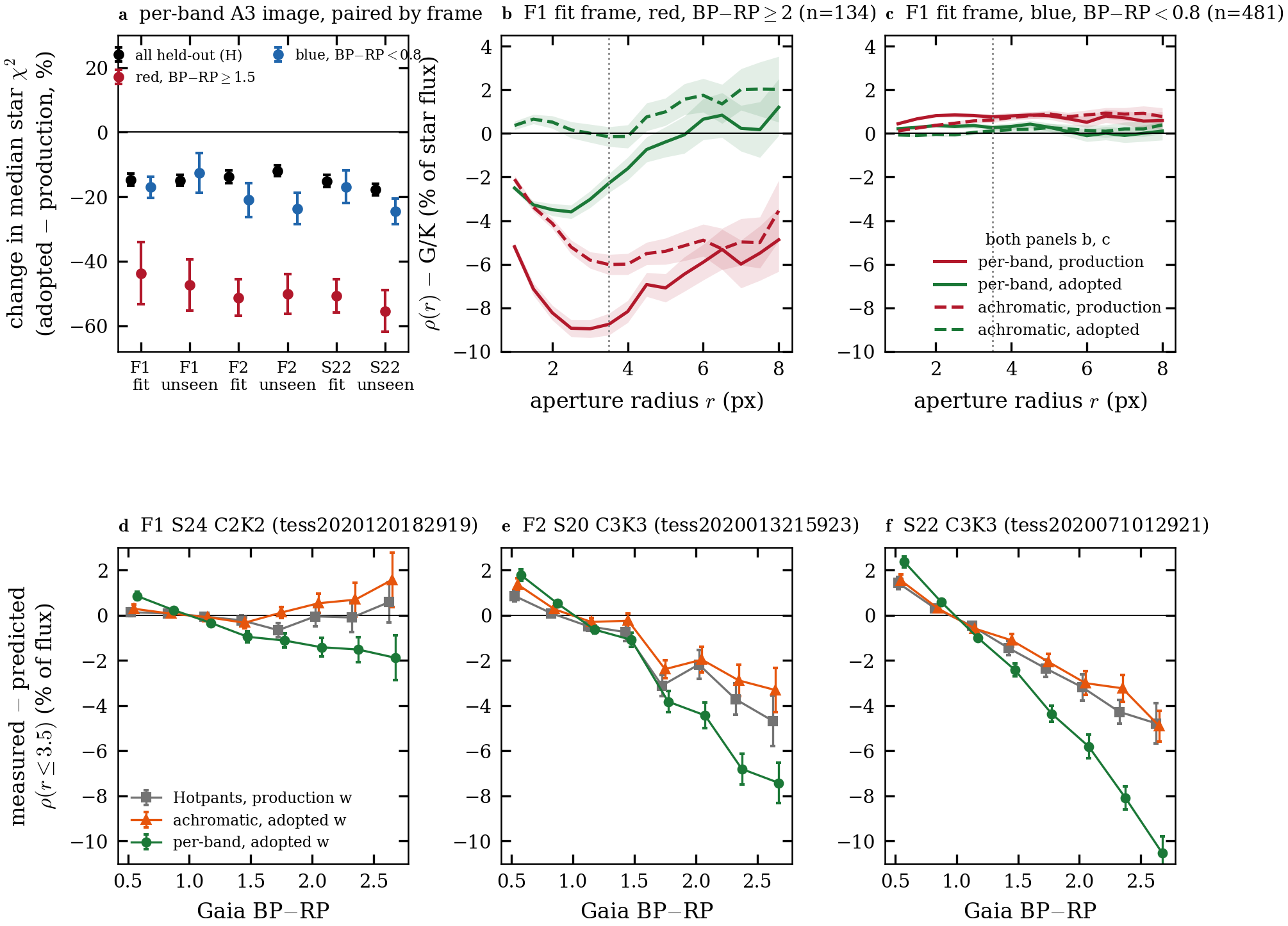
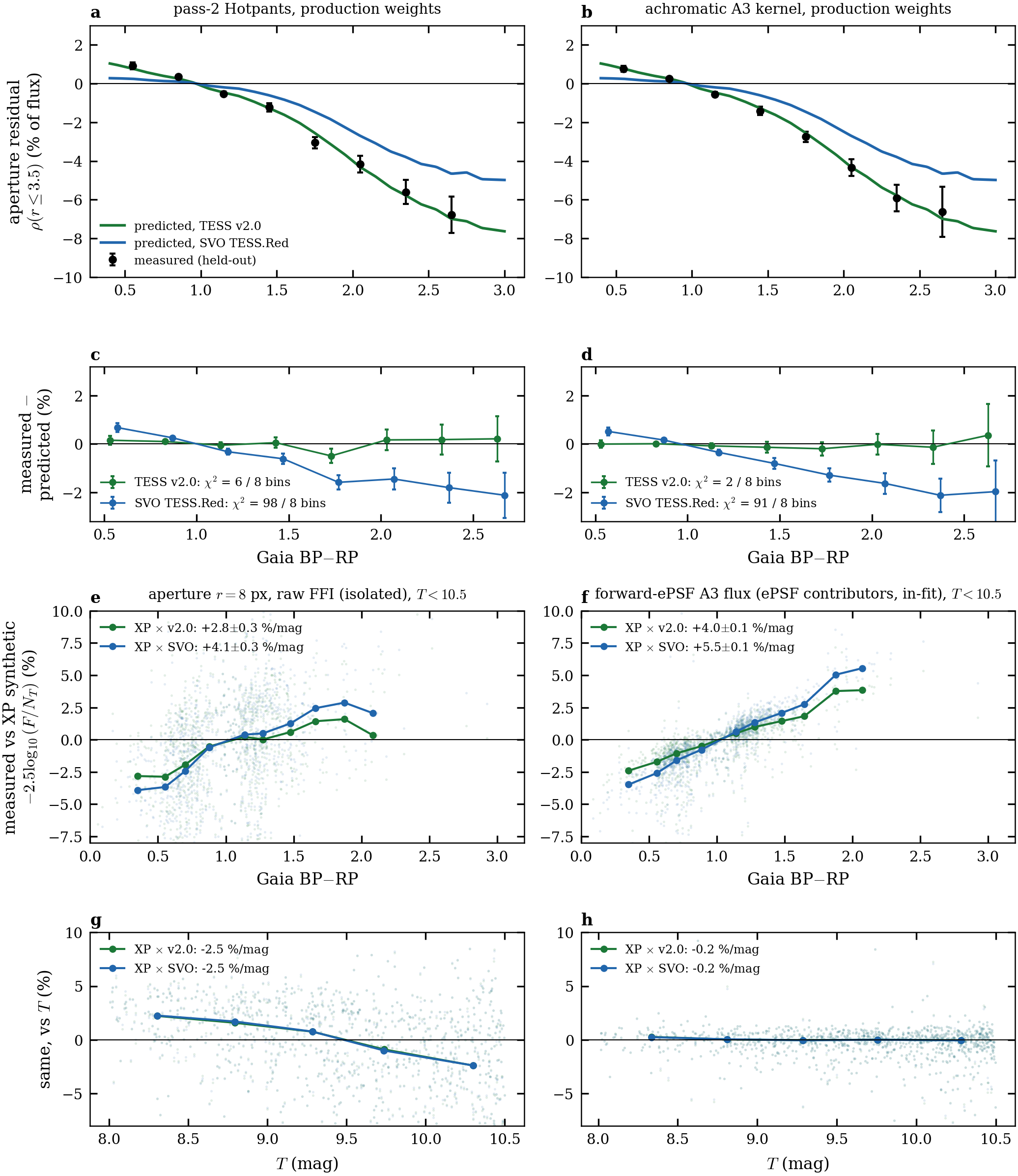
(a–d) Held-out 13 ≤ T < 16 stars in the adopted frame, production weights, no free parameters. The measured red−blue aperture residual follows the v2.0 synthesis-error prediction: χ² = 6 (Hotpants) and 2 (achromatic A3 kernel) over 8 colour bins, against 98 and 91 for SVO. The per-band column is omitted because A3's red sharpening confounds it. (e–h) Bright stars with T < 10.5. The colour slope is smaller with v2.0 (apertures +2.8 vs +4.1 %/mag; forward-ePSF +4.0 vs +5.5 %/mag, contributors in-fit), and the Tmag term is identical under both curves. Panel g's −2.5 %/mag Tmag term is the aperture sky bias.
(a) Paired change from production to adopted weights in the per-band A3 image, for the fit and unseen frames of each field. The median star χ² falls on every frame: about 15% for all held-out stars, 45–55% for red stars (BP−RP ≥ 1.5) and 12–25% for blue stars. (b, c) F1: enclosed residual $\rho(r)$ with the G/K median removed. For red stars (BP−RP ≥ 2) at r = 3.5 px it goes from −8.8% to −2.3% (per-band) and from −6.0% to −0.2% (achromatic); blue stars are within 1% in both. (d–f) Measured minus predicted $\rho(r\leq3.5)$, with no free parameters. F1 follows the v2.0 prediction (Hotpants χ² 8.6 over 8 bins). On F2 and S22, both camera 3 / CCD 3, red stars stay fainter than predicted in every product including Hotpants (χ² 125 and 233), so the adopted weights cannot remove it there. On top of that CCD-level deficit, the per-band product carries an A3 red-sharpening core, and that core is larger on C3K3. Per-band minus achromatic at BP−RP 2.35 / 2.65 is −2.2 / −3.4% on F1, −3.9 / −4.1% on F2, and −4.9 / −5.6% on S22. How the paper handles C3K3 is pending your decision. All stars are held-out, 13 ≤ T < 16.